Principal Component Analysis

Direction of maximum variance

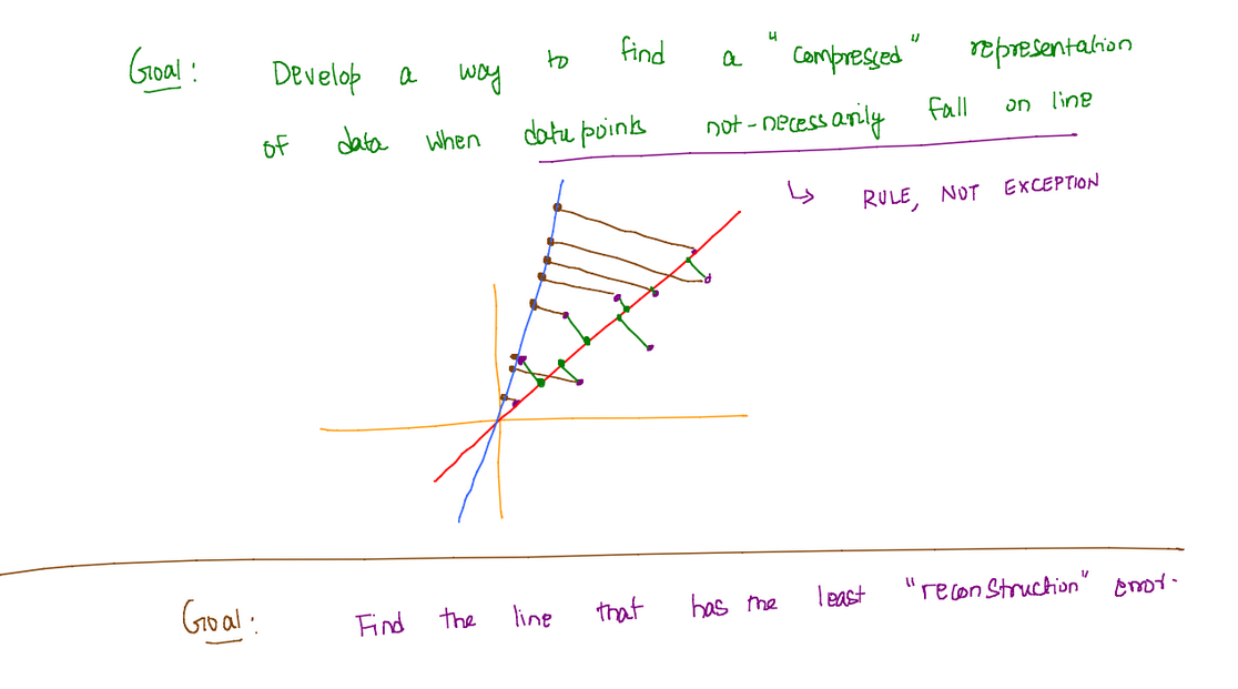
Let’s say we have a set of datapoints for which we wish to obtain a “compressed” representation using a line. The line that can best act as a representative for these data points must have the minimum reconstruction error.

For any datapoint $x_i$ and the representative line $w$, the representation of $x_i$ on $w$ is the projection of $x_i$ on $w$, i.e. $(x_i^{T}w)w$.

To find such a $w$, we wish to obtain $\arg \min Error(Line,Dataset)$ where,

$$\begin{array}{rl}Error(Line,Dataset)& =\frac{1}{n}\sum _{i=1}^n\mathrm{length}(x_i-(x_i^{T}w)w)\\ & =\frac{1}{n}\sum _{i=1}^n(x_i-(x_i^{T}w)w{)}^T(x_i-(x_i^{T}w)w)\\ & =\frac{1}{n}\sum _{i=1}^n\left[x_i^T{x}_i-(x_i^{T}w{)}^2-(x_i^{T}w{)}^2+(x_i^{T}w{)}^2{w}^{T}w\right]\\ & =\frac{1}{n}\sum _{i=1}^n\left[x_i^T{x}_i-(x_i^{T}w{)}^2\right](\text{If w is a unit vector})\end{array}$$

In this above error term, the $x_i^T{x}_i$ term is independent of $w$. Thus the error can be re-written as,

$$\begin{array}{r}Error(Line,Dataset)=\frac{1}{n}\sum _{i=1}^n-(x_i^{T}w{)}^2\end{array}$$

And thus the optimization problem can becomes a maximization of error instead.

$$\begin{array}{rl}\arg \max & Error(Line,Dataset)\\ Error(Line,Dataset)& =\frac{1}{n}\sum _{i=1}^n(x_i^{T}w{)}^2\\ & =\frac{1}{n}\sum _{i=1}^n(w^T{x}_i)(x_i^{T}w)\\ & =\frac{1}{n}\sum _{i=1}^n{w}^T(x_i{x}_i^T)w\\ & =w^T\left(\frac{1}{n}\sum _{i=1}^n(x_i{x}_i^T)\right)w\\ & =w^T{\Sigma }_{x}w\end{array}$$

Where ${\Sigma }_x$ is the covariance matrix for the random vector $[x_1,x_2,\dots ,x_n]$. If we recall the properties of the covariance matrix, we can see that the above form of the error function heavily resembles the variance of a random vector.

Also notice how the formula we arrive at is similar to the covariance formula for a random vector, with just the mean being 0. This means that centering the data is essential for variance maximization.

Thus the best representative line $w$ will be the one that captures that maximum variance in the dataset.

Residual Analysis

The residue left after determining a representation for $x_i$ need not be error. It can still hold some information crucial for a full reconstruction of the original dataset.

Some observation about the residues -

1. All residues are orthogonal to the first representation $w_1$.
2. Any line which minimizes the sum of errors w.r.t the residuals must also be orthogonal to $w_1$ as all such lines would lie in the orthogonal complement of $w_1$.

If $\{x_1,x_2,\dots ,x_n\}$ are our original datapoints, the residues left after representing them using $w_1$ would be

$$\{x_1-(x_1^T{w}_1)w_1,x_2-(x_2^T{w}_1)w_1,\dots ,x_n-(x_n^T{w}_1)w_1\}$$

We can then find another line in the orthogonal complement of $w_1$ which would minimize the sum of errors w.r.t these residuals and yield us new residues $-$

$$\begin{array}{rlr}& & \{x_1-(x_1^T{w}_1)w_1-((x_1-(x_1^T{w}_1)w_1{)}^T{w}_2)w_2\}\\ & \Rightarrow & \{x_1-(x_1^T{w}_1)w_1-(x_1^T{w}_2-(x_1^T{w}_1)w_1^T{w}_2)w_2\}\\ & \Rightarrow & \{x_1-(x_1^T{w}_1)w_1-(x_1^T{w}_2)w_2\}\end{array}$$

Thus the residue after $d$ rounds would be,

$$\left\{x_1-\sum _{i=1}^d(x_1^T{w}_1)w_1=\vec{0}\right\}$$

because after $d$ rounds, we’d be left with $d$ orthonormal basis which would span all of ${\mathbb{R}}^d$.

Note - If the datapoints lie in a low dimensional subspace of ${\mathbb{R}}^d$ then the residues would become 0 much earlier than $d$ rounds.

For any $w\in {\mathbb{R}}^d$, such that $||w|{|}_2^2=1$

$$\begin{array}{rlrl}& & ||x_i|{|}^2& =||x_i-(x_i^{T}w)|{|}^2+||(x_i^{T}w)w|{|}^2\\ & \Rightarrow & ||x_i|{|}^2& =\underset{\text{Error}}{\underbrace{||x_i-(x_i^{T}w)|{|}^2}}+\underset{\text{Representation}}{\underbrace{||(x_i^{T}w)w|{|}^2}}\end{array}$$

We want this representation term to be as large as possible for a better fit.

Eigenvalues of the Covariance Matrix

The optimization problem discussed above can be solved using the Hilbert’s Min-Max Theorem. This tells us that $w_1$ is the eigenvector of ${\Sigma }_x$ corresponding to the largest eigenvalue of ${\Sigma }_x$.

If $w_1$ is an eigenvector of ${\Sigma }_x$, we can say that

$$\begin{array}{rlrlr}& & {\Sigma }_x{w}_1& ={\lambda }_1{w}_1& \\ & \Rightarrow & w_1^T{\Sigma }_x{w}_1& =w_1^T{\lambda }_1{w}_1& \\ & \Rightarrow & w_1^T{\Sigma }_x{w}_1& ={\lambda }_1& \because w^{T}w=1\\ & \Rightarrow & {\lambda }_1& =w_1^T\frac{1}{n}\sum _{i=1}^n(x_i{x}_i^T)w_1& \\ & \Rightarrow & {\lambda }_1& =\frac{1}{n}\sum _{i=1}^n(x_i^T{w}_1{)}^2& \end{array}$$

This is exactly the optimization error term we used earlier to restructure the error as variance. Thus we can say that the largest eigenvalue of the covariance matrix is literally the variance of the data projected onto $w_1$.

Because the covariance matrix is symmetric, the eigenvectors for it will be orthogonal. Thus the eigenvector $w_2$ corresponding to the second highest eigenvalue ${\lambda }_2$ will naturally lie in the orthogonal complement of $w_1$ and ${\lambda }_2$ would correspond to the variance of the data projected onto $w_2$.

Sequentially, all eigenvalues of the covariance matrix would in-turn correspond to the variance of the data projected onto the eigenvector corresponding to them.

Rule of thumb for dimensions

The most common assumption is that any data point $x_i$ is made up of two components. The actual signal $s_i$ and the random noise ${ϵ}_i$. Because this noise is random in nature, it doesn’t have a particular pattern which it follows. It has not preferred direction, tends to be small in magnitude, and contributes a small and roughly equal amount of variance in every direction.

Thus by looking at the eigenvalues of our covariance matrix, we can say that the smaller eigenvalues may correspond to this random noise and the eigenvectors corresponding to these eigenvalues are redundant for a proper reconstruction of the original data. So instead of trying to capture all the variance in our original data, we can only use some top $k$ eigenvalues and their corresponding eigenvectors to capture some $t$ threshold of variance, typically 0.95.

We can identify our top $k$ directions by doing $-$

$$\frac{{\sum }_{i=1}^k{\lambda }_i({\Sigma }_x)}{{\sum }_{i=1}^d{\lambda }_i({\Sigma }_x)}\ge 0.95$$

Because all eigenvalues correspond to variance which is non-negative, this summation will be non-decreasing.

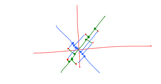
Let the green line represent $w_1$ and the blue line represent $w_2$. Notice how the variance of the data along $w_1$ is much more than the variance of the data on $w_2$.