VDM and GANs

Table of Contents

• Deep Generative Models
• Variational Divergence Minimization
  • f-divergence
  • Algorithm for f-divergence minimization
    • Conjugate of a convex function
  • Realization of VDM (Variational Divergence Minimization)
  • Implementing VDM for Generative Modelling
• Generative Adversarial Networks
  • Implementation of GAN in practice
    • To train the Discriminator
    • To Train the Generator
  • Interpretation of GANs as Classifier guided Generative Samplers
    • Formulation of classifier guided sampler
• Deep Convolution GAN (DC Gan)
• Conditional GAN (cGAN)
• VDM
• Improvisations and Applications of GANs
  • Wasserstein’s GANs (WGANs)
    • What makes GAN training unstable?
    • Wasserstein’s Metric (Optimal Transport)
    • How to minimize Wasserstein’s Metric
  • Bi-Directional GAN (Bi-GAN)
    • Inversion of GANs
    • Bi-Directional GAN
  • Domain Adversarial Networks
  • Evaluation of a GAN

Deep Generative Models

Family of Deep Generative Models (DGMs) to be covered -

1. Generative Adversarial Networks (GANs)
2. Variational Auto Encoders (VAEs)
3. Denoising Diffusion Probabilistic Models (DDPMs)
   • Score Based Models
4. Auto Regressive Models (AR)
   • Large Language Models (LLMs)
5. State Space Models (SSMs)
   • Example - S4, Mamba
6. RL-based Alignment for LLMs
   • RLHF, PPO, DPO

Any dataset $D=\{x_i{\}}_{i=1}^n,X_i\stackrel{\text{i.i.d}}{\sim }{\mathbb{P}}_x,x_i=X_i(\omega ),x_i\in {\mathbb{R}}^d$ means that $D$ consists of independent realizations of i.i.d. vector valued random variables $X_1,X_2,\dots$ of size $d$, each distributed according to some unknown probability distribution ${\mathbb{P}}_X$.

Goal - Given such a $D$, the goal of using Generative Models is to estimate ${\mathbb{P}}_X$ and learn to sample from it.

Principles of Generative Models -

1. Assume a parametric family on ${\mathbb{P}}_X$ denoted using ${\mathbb{P}}_{\theta }$ where ${\mathbb{P}}_{\theta }$ is represented using Deep Neural Networks. This is our “model”.
2. Define and estimate a divergence metric to measure the distance between ${\mathbb{P}}_X$ and ${\mathbb{P}}_{\theta }$.
3. Solve an optimization problem over the parameters of ${\mathbb{P}}_{\theta }$ to minimize the divergence metric.

Example

Assume some random variable $z$ with some arbitrary but known distribution $Z$ (because the distribution is known, sampling is possible). Suppose there exists some function $g_{\theta }(z):Z\to X$.

• $\tilde{x}=g_{\theta }(z)$ would have an entirely different distribution that that of $z$ and would depend upon the function $g_{\theta }$.
• Suppose $g_{\theta }(z)$ is a Deep Neural Network and the density of $\tilde{x}=g_{\theta }(z)$ is denoted as ${\mathbb{P}}_{\theta }$. We can define a divergence metric $D({\mathbb{P}}_X||{\mathbb{P}}_{\theta })$ between ${\mathbb{P}}_{\theta }$ and ${\mathbb{P}}_X$ such that $D({\mathbb{P}}_X||{\mathbb{P}}_{\theta })\ge 0$ and $D({\mathbb{P}}_X||{\mathbb{P}}_{\theta })=0$ iff ${\mathbb{P}}_X={\mathbb{P}}_{\theta }$.
• Solving the optimization equation ${\theta }^{\ast }=\arg {\min }_{\theta }D({\mathbb{P}}_X||{\mathbb{P}}_{\theta })$, would allow us to implicitly estimate ${\mathbb{P}}_X$. This would allow us to sample from ${\mathbb{P}}_X$ using $g_{\theta \ast }(z)$ because a random sample chosen from $z$ and then passed through $g_{\theta \ast }(z)$ would be very close to ${\mathbb{P}}_X$.

This method is called a pushforward method as we push a probability mass $Z$ into the data space $X$ using a function $g_{\theta }$.

Obstacles towards implementation -

1. We know random samples from these distributions, the dataset $D$ from ${\mathbb{P}}_X$ and $g_{\theta }(z)$ from ${\mathbb{P}}_{\theta }$, but not the distributions themselves. How to compute the divergence metric without knowing the distributions ${\mathbb{P}}_X$ and ${\mathbb{P}}_{\theta }$?
2. What should the choice of the divergence metric be?
3. How to choose $g_{\theta }$ and in turn ${\mathbb{P}}_{\theta }$?
4. How to solve the optimization problem of minimizing the divergence metric?

Variational Divergence Minimization

Define a diverge between two distributions

f-divergence

Given two probability distribution functions with corresponding probability density functions denoted by $P_X$ and $P_{\theta }$, the f-divergence between them is -

$$\begin{array}{rl}& D_f(P_X||P_{\theta })={\int }_X{P}_{\theta }(x)f\left(\frac{P_X(x)}{P_{\theta }(x)}\right)dx\\ & f(u):{\mathbb{R}}^{+}\to \mathbb{R}\text{ is a convex, left semi-continous and }f(1)=0(\text{any function})\\ & x:\text{space on which }{P}_X\text{ and }{P}_{\theta }\text{ are supported}\end{array}$$

• Convex function - A function which has one unique minimum value (can have multiple minima).
• Strictly Convex function - A function which has only one global minima.
• Left Semi-Continuous function - A function in which the value at a point is equal to the limit when approached from the left.
• Probability density functions are always non-negative, thus their ratio $\frac{P_X(x)}{P_{\theta }(x)}$ will be a positive value which would satisfy the domain of $f$.
• Range space of $P_X$ and $P_{\theta }$ would be positive scalars despite $x$ being a $d$-dimensional random vector.

Choice of an $f$ function is what leads to an $f$-divergence.

Properties of $f$-divergence -

1. $D_f\ge 0$ for any choice of $f$.
2. $D_f(P_X||P_{\theta })=0$ iff $P_X=P_{\theta }$.

Examples of $f$-divergence -

1. $f(u)=ulogu$ leads to the KL (Kullback-Leilber) Divergence -

$${\int }_X{P}_X(x)log\left(\frac{P_X(x)}{P_{\theta }(x)}\right)dx=D_{KL}$$

K.L Divergence is asymmetric, meaning $\underset{\text{Forward K.L.}}{\underbrace{D(P_X||P_{\theta })}}\ne \underset{\text{Reverse K.L.}}{\underbrace{D(P_{\theta }||P_X)}}$.

2. $f(u)=\frac{1}{2}\left(ulogu-(u+1)log\left(\frac{u+1}{2}\right)\right)$ leads to the JS (Jensen-Shannon) Divergence.
3. $f(u)=\frac{1}{2}|u-1|$ leads to the Total Variation Distance or TV Distance.

Algorithm for f-divergence minimization

We need to come up with an algorithm to optimize the $f$-divergence without knowing what the distributions $P_X$ and $P_{\theta }$ are but instead by using the samples of $P_X$ and $P_{\theta }$ known to us (dataset $D$ and output of $g_{\theta }(z)$).

Key Idea - Integrals involving density functions can be approximated using samples drawn from the distribution.

For an integral like the one shown below, we have i.i.d samples drawn from $P_X$.

$$I={\int }_{X}h(x)P_x(x)dx$$

$(1)$ By the Law of Unconscious Statistician (LOTUS) we know that if $X$ is a random variable with a probability distribution $P_X$ and $h$ is some measurable function, then

$${\int }_{X}h(x)P_x(x)dx={\mathbb{E}}_{P_X}(h(x))$$

$(2)$ By the Law of Large Numbers, we know that as the number of samples grows, the sample mean converges to the true expected value of a function $h$.

$$\underset{n\to \infty }{\lim }\frac{1}{n}\sum _{i=1}^{n}h(x_i)\approx \mathbb{E}[h(x)]$$

So one way to solve an integral like the f-Divergence is by using the above two mentioned laws and equating it to the expected value of function $h(x)=f\left(\frac{P_X(x)}{P_{\theta }(x)}\right)$. It would be a mathematically valid representation but is not directly computable from the data since the true data distribution $P_X$ is unknown.

Conjugate of a convex function

The conjugate of a convex function $f(u)$ is written as

$$f^{\ast }(t)=\underset{u\in \text{dom(f)}}{\sup }\left\{ut-f(u)\right\}$$

At every point $t$, one constructs multiple lower bounds on that particular $u$ and chooses the tightest of those lower bounds (supremum/max) as value of the conjugate.

Properties of a conjugate of a convex function -

1. $f^{\ast }$ is also a convex function.
2. ${\left[f^{\ast }(t)\right]}^{\ast }=f(u)$

Using these properties of a conjugate of a convex function, we can write $f(u)$ as -

$$f(u)=\underset{t\in \text{dom(f*)}}{\sup }\left\{tu-f^{\ast }(t)\right\}$$

Substituting this in the f-Divergence Integral we get -

$$\begin{array}{rlr}{D}_f(P_X||P_{\theta })& ={\int }_X{P}_{\theta }(x)f\left(\underset{u}{\underbrace{\frac{P_X(x)}{P_{\theta }(x)}}}\right)dx& \\ & ={\int }_X{P}_{\theta }(x)f(u)dx& \because u=\frac{P_X(x)}{P_{\theta }(x)}\\ & ={\int }_X{P}_{\theta }(x)\underset{t\in \text{dom(f*)}}{\sup }\left\{t\ast \frac{P_X(x)}{P_{\theta }(x)}-f^{\ast }(t)\right\}dx& \end{array}$$

To represent the $f$-divergence in terms of expectation, we need to somehow take the supremum out of the integral. Since the Fenchel conjugate expresses $f(u)$ as a pointwise supremum, and since $u=\frac{P_X(x)}{P_{\theta }(x)}$​ depends on $x$, the optimizer of the inner problem is generally a function of $x$. Thus we can take the supremum out and rewrite the equation as -

$$\begin{array}{rlr}& =\underset{T(x)\in \text{T}}{\sup }{\int }_X{P}_{\theta }(x)\left\{T(x)\ast \frac{P_X(x)}{P_{\theta }(x)}-f^{\ast }(T(x))\right\}dx& \end{array}$$

where $\mathbb{T}:X\to \text{dom f*}$ is the space of functions containing solutions for the inner optimization problem.

The space of functions $\mathbb{T}$ we are optimizing over may or may not containing $T^{\ast }(x)$ that is the solution to the inner optimization problem. This can occur either because $\mathbb{T}$ is a restricted function class (e.g., neural networks), or because the supremum defining the conjugate is not attained within $\mathbb{T}$.

Because we are restricting $\mathbb{T}$ and $\mathbb{T}\subseteq \{\text{all measurable functions}\}$, by using the fact for any arbitrary function $F$ that ${\sup }_{t\in A}F(x)\le {\sup }_{t\in B}F(x)$ if $A\subseteq B$ we can say,

$$\begin{array}{rl}{D}_f& \ge \underset{T(x)\in \text{T}}{\sup }{\int }_X{P}_{\theta }(x)\left\{T(x)\ast \frac{P_X(x)}{P_{\theta }(x)}-f^{\ast }(T(x))\right\}dx\\ & \ge \underset{T(x)\in \text{T}}{\sup }{\int }_X{P}_X(x)T(x)dx-{\int }_X{P}_{\theta }(x)f^{\ast }(T(x))dx\\ D_f& \ge \boxed{\underset{T(x)\in \text{T}}{\sup }[\underset{P_X}{\mathbb{E}}[T(x)]-\underset{P_{\theta }}{\mathbb{E}}[f^{\ast }(T(x))\left]\right]}\end{array}$$

For the sake of understanding, we can replace $\sup$ in the above equation with $\max$.

$$D_f\ge \underset{T(x)\in \text{T}}{\max }[\underset{P_X}{\mathbb{E}}[T(x)]-\underset{P_{\theta }}{\mathbb{E}}[f^{\ast }(T(x))\left]\right]$$

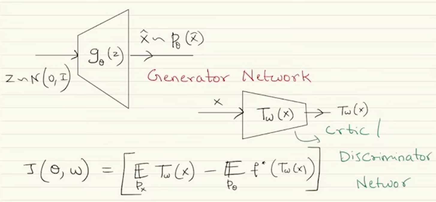
Realization of VDM (Variational Divergence Minimization)

We need a ${\theta }^{\ast }$ that minimizes the $f$-divergence $D_f$. $D_f$ is not optimizable due to $P_X$ being unknown. At the true optimum ${\theta }^{\ast }$ the lower bound on $D_f$ becomes a tight bound, thus making the optimization of $D_f$ and the optimization of the lower bound equivalent.

$$\begin{array}{rl}{\theta }^{\ast }& =\arg \underset{\theta }{\min }{D}_f\\ & \approx \arg \underset{\theta }{\min }\left[\text{lower bound of }{D}_f\right]\\ & =\arg \underset{\theta }{\min }\left[\underset{T(x)\in \text{T}}{\max }\right[\underset{P_X}{\mathbb{E}}[T(x)]-\underset{P_{\theta }}{\mathbb{E}}[f^{\ast }(T(x))]\left]\right]\end{array}$$

The final objective here requires two optimizations -

1. Generator Network - The outer minimization w.r.t parameters of $g_{\theta }(z)$.
2. Critic/Discriminator Network - The inner maximization w.r.t a class of functions $T(x)\in \mathbb{T}$.

With this the objective becomes -

$${\theta }^{\ast },w^{\ast }=\arg \underset{\theta }{\min }\underset{w}{\max }[\underset{P_X}{\mathbb{E}}[T_w(x)]-\underset{P_{\theta }}{\mathbb{E}}[f^{\ast }(T_w(x))\left]\right]$$

Neural networks enter the framework when we need to perform the saddle-point optimization of the variational lower bound of the $f$-divergence, since both the generator distribution and the variational function are infinite-dimensional objects.

• The model distribution $P_{\theta }$ must be learnt to reduce the value of the $f$-divergence metric. Neural networks provide a flexible and differentiable parameterization for learning such complex data-generating distributions using the samples.
• The function class $\mathbb{T}$, being infinite dimensional, is difficult to characterize explicitly. As neural networks are universal function approximators, we represent $\mathbb{T}$ using neural networks $T_w(x)$ where $w$ are the parameters of the neural network.

Implementing VDM for Generative Modelling

Now we have two neural networks, one representing the sampler (Generator Network) and the other representing the $\mathbb{T}$ function class (Critic Network).

$$\begin{array}{rl}J(\theta ,w)& =\underset{P_X}{\mathbb{E}}[T_w(x)]-\underset{P_{\theta }}{\mathbb{E}}[f^{\ast }(T_w(x))]\\ {\theta }^{\ast },w^{\ast }& =\arg \underset{\theta }{\min }\underset{w}{\max }J(\theta ,w)\end{array}$$

Such problems are called a saddle-point optimization problems as we are looking for saddle points here or an adversarial optimization problem because whatever one network is trying to do is the opposite of what the other network is trying to do.

Usually we avoid saddle-points because they are neither a global minima nor a global maxima, but this is one of the rare instances where we seek a saddle point.

By construction $T_w:X\to \mathrm{dom}{f}^{\ast }$ is dependent upon the particular choice of $f$. $T_w$ can be rewritten as $T_w={\sigma }_f(V_w(x))$ to guarantee that the critic’s output lies in the domain of $f^{\ast }$ while keeping the network architecture independent of our choice of the $f$-divergence. Here -

• $V_w(x):X\to \mathbb{R}$ is a function common across all $f$-divergence
• ${\sigma }_f(v):\mathbb{R}\to \mathrm{dom}{f}^{\ast }$ is an $f$-divergence specific activation function (need not always be the sigmoid function)

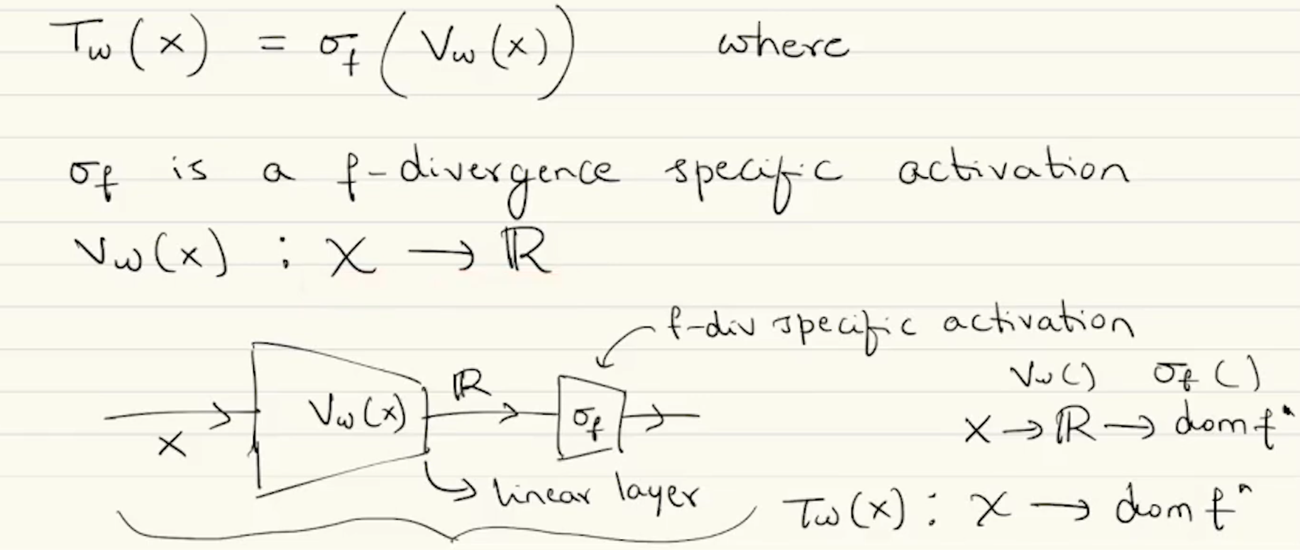
So we can rewrite our loss function as -

$$J(\theta ,w)=\underset{P_X}{\mathbb{E}}[{\sigma }_f(V_w(x))]-\underset{P_{\theta }}{\mathbb{E}}[f^{\ast }({\sigma }_f(V_w(x)))]$$

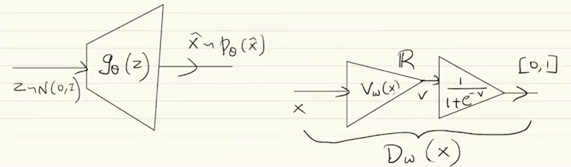
Generative Adversarial Networks

For GANs the $f$-divergence that is chosen is as follows -

$$\begin{array}{rlr}f(u)& =ulogu-(u+1)log(u+1)& \text{(Similar to }f\text{ used in JS-divergence)}\\ f^{\ast }(t)& =-log(1-exp(t)),& \mathrm{dom}{f}^{\ast }={\mathbb{R}}^{-}\\ {\sigma }_f(v)& =-log(1+e^{-v})& \text{(log-sigmoid)}\end{array}$$

The log-sigmoid as ${\sigma }_f$ ensures that the output of the critic always lies in $\mathrm{dom}{f}^{\ast }={\mathbb{R}}^{-}$. Using the above information, we can write a GAN specific loss function using the equation of a loss function we got earlier.

$$\begin{array}{rl}{J}_{GAN}(\theta ,w)& =\underset{P_X}{\mathbb{E}}[log{D}_w(x)]+\underset{P_{\theta }}{\mathbb{E}}[log(1-D_w(x))]\\ \text{where}{D}_w(x)& =\frac{1}{1+e^{-V_w(x)}}\text{(the sigmoid function}\&D_w(x)\in \{0,1\})\end{array}$$

Observations to note -

• Due to the rearrangement of terms again satisfying the lower-bound equation, we can see that $T_w(X)=log{D}_w(x)$.
• It can also be seen that this objective function strangely resembles the cross-entropy loss.
• The discriminator would try to maximize this “cross-entropy” by maximizing the objective function. Since the cross-entropy is large when real and fake samples are easily distinguishable, maximizing it encourages the discriminator to separate samples from $P_X$​ and $P_{\theta }$​ as effectively as possible. Thus it is called the “discriminator.”
• The generator would try to minimize this “cross-entropy” by only minimizing the second term of the objective function. In general this second term penalizes incorrect predictions made with a high probability. In this case it would be penalizing the fake samples the discriminator confidently distinguishes as fake. By minimizing it, the generator encourages the discriminator to assign higher probabilities to generated samples, which implicitly pushes the generator distribution $P_{\theta }$​ towards the data distribution $P_X$​.
• The above two observations are solidifying more in Formulation of classifier guided sampler.
• The discriminator is trying to assign a low probability to the generated samples while the generator pushes the discriminator to assign them a high probability. This causes the adversarial nature of the networks.

The architecture ends up looking like the image below. $log$ doesn’t need to be included in the discriminator network as it is not a part of the networks but the error function.

Implementation of GAN in practice

Pre-requisites -

• Input $D=\{x_1,x_2,\dots \}\stackrel{\text{i.i.d}}{\sim }{P}_X$.
• Let $B_1=\{x_1,x_2,\dots ,x_{B_1}\}\subset D$ (need not be contiguous, is usually random) be a mini-batch taken from the dataset.
• Let $B_2=\{z_1,z_2,\dots ,z_{B_2}\}$ be a batch of random noise vectors taken from the arbitrary distribution we chose, typically $\mathcal{N}(0,1)$.

As we are using these batches during Mini-Batch gradient descent, these batches are resampled each time before an update.

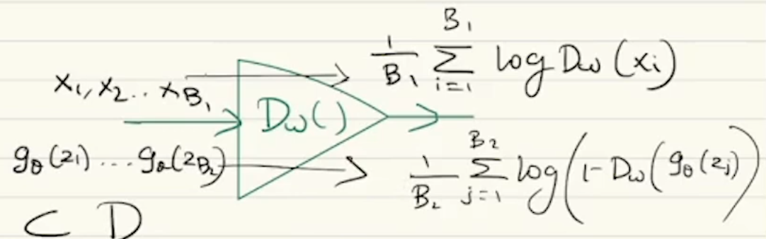
To train the Discriminator

Optimizing for $w$ -

$$\begin{array}{rl}{w}^{\ast }& =\arg \underset{w}{\max }{J}_{GAN}(\theta ,w)\\ & =\arg \underset{w}{\max }[\underset{P_X}{\mathbb{E}}[log{D}_w(x)]+\underset{P_{\theta }}{\mathbb{E}}[log(1-D_w(x))]]\\ & \approx \arg \underset{w}{\max }[\frac{1}{B_1}\sum _{i=1}^{B_1}log{D}_w(x_i)+\frac{1}{B_2}\sum _{i=1}^{B_2}log(1-D_w({\hat{x}}_i))]\because \text{Using batch size}\end{array}$$

Steps -

1. Resample $B_1$ and $B_2$.
2. Pass $x_i\in B_1$ through the discriminator $D_w$ to get $D_w(x_i)$. Then using these calculate the first term of the loss function -

$$\frac{1}{B_1}\sum _{i=1}^{B_1}log{D}_w(x_i)$$

3. Keeping $\theta$ constant, pass the random noise vectors $z_i\in B_2$ through the generator to generate fake samples ${\hat{x}}_i=g_{\theta }(z_i)$. Pass this through the discriminator to get $D_w({\hat{x}}_i)$. Using these calculate the second term of the loss function -

$$\frac{1}{B_2}\sum _{i=1}^{B_2}log(1-D_w({\hat{x}}_i))$$

4. Calculate the gradient $\underset{w}{\nabla }{J}_{GAN}(\theta ,w)$ and backpropagate the gradients back through the discriminator network.
5. Update $w$ using gradient “ascent”.

$$w^{t+1}=w^t+{\alpha }_1\underset{w}{\nabla }{J}_{GAN}(\theta ,w)$$

To Train the Generator

Optimizing for $\theta$ -

$$\begin{array}{rl}{\theta }^{\ast }& =\arg \underset{\theta }{\min }{J}_{GAN}(\theta ,w)\\ & =\arg \underset{\theta }{\min }[\underset{P_X}{\mathbb{E}}[log{D}_w(x)]+\underset{P_{\theta }}{\mathbb{E}}[log(1-D_w(x))]]\\ & \approx \arg \underset{\theta }{\min }[{\cancel{\frac{1}{B_1}\sum _{i=1}^{B_1}log{D}_w(x_i)}}^{\text{Independent of }\theta }+\frac{1}{B_2}\sum _{i=1}^{B_2}log(1-D_w({\hat{x}}_i))]\\ & =\arg \underset{\theta }{\min }[\frac{1}{B_2}\sum _{i=1}^{B_2}log(1-D_w({\hat{x}}_i)]\because \text{Second term stays as }{\hat{x}}_i=g_{\theta }(z_j)\in P_{\theta }\end{array}$$

Steps -

1. Resample $B_2$.
2. Keeping $w$ constant, pass the random noise vectors $z_i\in B_2$ through the generator to generate fake samples ${\hat{x}}_i=g_{\theta }(z_i)$. Pass this through the discriminator to get $D_w({\hat{x}}_i)$. Using these calculate the term of the loss function -

$$\frac{1}{B_2}\sum _{i=1}^{B_2}log(1-D_w({\hat{x}}_i))$$

3. Calculate the gradient $\underset{\theta }{\nabla }{J}_{GAN}(\theta ,w)$ and backpropagate the gradients back through the discriminator network and then through the generator network. The discriminators parameters are not updated as $w$ is set to constant.
4. Update $\theta$ using gradient descent.

$${\theta }^{t+1}={\theta }^t-{\alpha }_2\underset{\theta }{\nabla }{J}_{GAN}(\theta ,w)$$

We have to solve these optimization problems alternatively. First update the generator parameters while keeping the discriminator parameters are constant, then update the discriminator parameters while keeping the generator parameters are constant.

Interpretation of GANs as Classifier guided Generative Samplers

In GANs the discriminator network $D_w$ acts as a binary classifier which is able to predict whether a given sample belongs to $P_X$ or $P_{\theta }$.

*Can this classifier be used to bring $P_X$ and $P_{\theta }$ closer?

• Yes! If $P_X$ and $P_{\theta }$ were sufficiently close to each other, even an optimal discriminator would fail to distinguish the samples between them. So we can tweak $\theta$ till the classifier fails to distinguish between samples of $P_X$ and $P_{\theta }$.
• However, the failure of some weak or arbitrary classifier doesn’t imply that $P_X$ and $P_{\theta }$ are close to each other. So instead of just tweaking $\theta$, we also need to change the binary classifier $D_w$. If all such different variations of the classifiers fail to distinguish the samples then we can confidently say that $P_X$ and $P_{\theta }$ are close to each other.

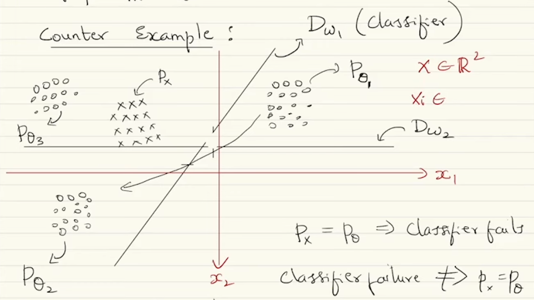
Mode Collapse Problem -

• During the updation of the generator and the classifier, it can happen that $\theta$ and the classifier keep alternating between two values and get stuck in an infinite loop. This is called the mode collapse problem.

Formulation of classifier guided sampler

Creating the classifier -

1. Let $D_w:\mathcal{X}\to [0,1]$ represent the probability of the sample $x$ coming from $P_X$.
2. We’d need to maximize the log-likelihood of $x$ coming from $P_X$ when $x\sim P_X$ (probability of real samples being marked as real) and also maximize the log-likelihood of $\hat{x}$ coming from $P_{\theta }$ when $\hat{x}\sim P_{\theta }$ (probability of fake samples being marked as fake). So the combined objective of the classifier becomes maximizing the sum of these two values.

$$\begin{array}{rl}\mathbb{E}[log{D}_w(x)]& :\text{log-likelihood that }x\sim P_X\\ \mathbb{E}[log(1-D_w(x))]& :\text{log-likelihood that }\hat{x}\sim P_{\theta }\\ w^{\ast }=\arg \underset{w}{\max }& [\underset{P_X}{\mathbb{E}}[log{D}_w(x)]+\underset{P_{\theta }}{\mathbb{E}}[log(1-D_w(\hat{x}))]]\end{array}$$

Similarly for the generator -

1. The objective for the generator is that the classifier has to “fail” in distinguishing samples from $P_X$ and $P_{\theta }$. So the goal here is to minimize the discriminator’s confidence that fake samples $\hat{x}$ coming from $P_{\theta }$ are fake.

$${\theta }^{\ast }=\arg \underset{\theta }{\min }[\underset{P_{\theta }}{\mathbb{E}}[log(1-D_w(\hat{x}))]]$$

Thus the overall objective becomes -

$${\theta }^{\ast },w^{\ast }=\arg \underset{\theta }{\min }\underset{w}{\max }[\underset{P_X}{\mathbb{E}}[log{D}_w(x)]+\underset{P_{\theta }}{\mathbb{E}}[log(1-D_w(\hat{x}))]]$$

Deep Convolution GAN (DC Gan)

(intentionally left incomplete for now)

Conditional GAN (cGAN)

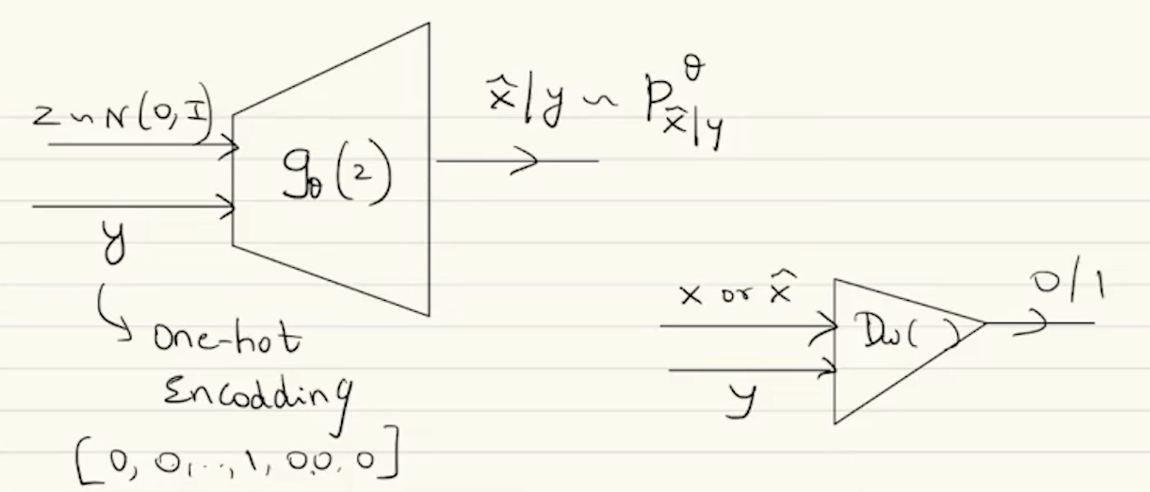
To make conditional GANs that sample from a conditional distribution, we pass the conditional variable $y$ through both the generator and the discriminator.

• Instead of just the noise $z\sim p(z)$ we pass $(z,y)$ so the generator learns $P_{\theta }(x|y)$.
• Instead of just seeing $x$, the discriminator sees $(x,y)\to D_w(x,y)$. It now answers “Is $x$ a real sample consistent with condition $y$“.

The objective function changes to -

$$J(\theta ,w)=\underset{(x,y)\sim P_{X|Y}}{\mathbb{E}}[log{D}_w(x)]+\underset{(\hat{x},y)\sim P_{\hat{X}|Y}}{\mathbb{E}}[log(1-D_w(\hat{x}))]$$

Inference with GANs/VDM

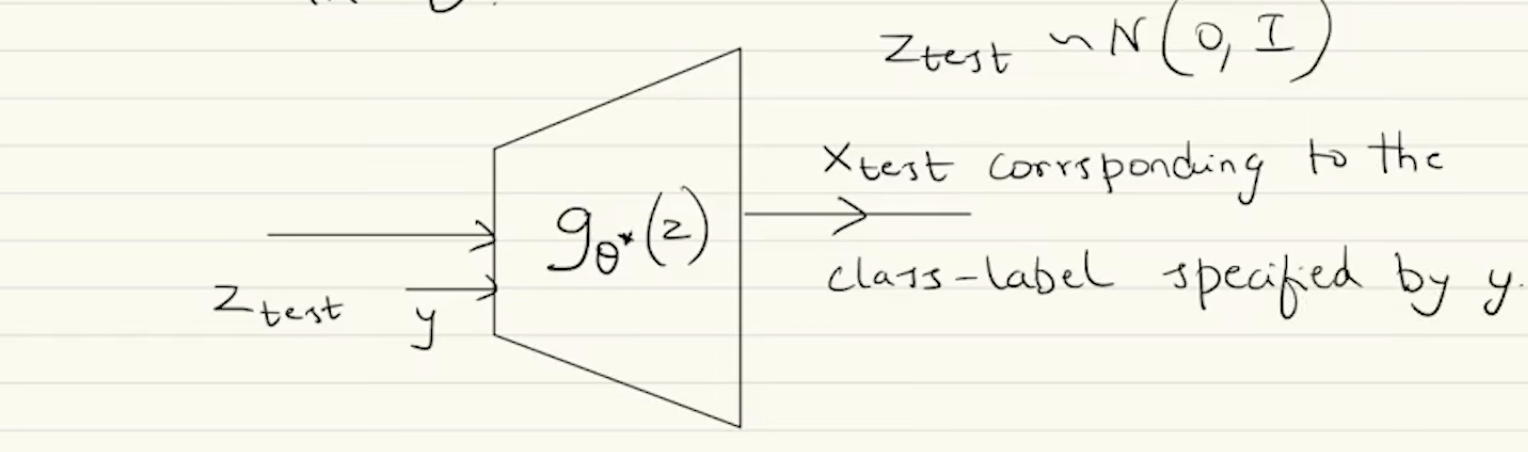
Suppose $g_{\theta }^{\ast }$ is the optimal generator network achieved via training. For any test input $z_{test}\sim \mathcal{N}(0,1)$ and class label $y$, the output would be a $X_{test}$ corresponding to the class-label specified by $y$.

Improvisations and Applications of GANs

Wasserstein’s GANs (WGANs)

What makes GAN training unstable?

Manifold Hypothesis -

• Images in the real world lie in a lower dimension manifold of the ambient space ${\mathbb{R}}^d$.
• Consider all $28\times 28$ images such that a pixel is 1 if a coin toss results in a heads, else 0. The probability of an image generated in such a manner resembling an English Alphabet is very low. So we can say that the images depicting an English Alphabet lie in a low dimensional manifold on the ambient space $\{0,1{\}}^{784}$.
• Similarly an image of any natural object lies in a lower dimension manifold of the image’s dimension ${\mathbb{R}}^d$.

The real distribution $P_X$ and the generated distribution $P_{\theta }$ are both distributions over ${\mathbb{R}}^{784}$. Since the real data and the generated data would lie over a lower dimensional manifold of ${\mathbb{R}}^d$, the supports (set on which the corresponding density function has a non-zero value) of $P_X$ and $P_{\theta }$ would misalign with a very high probability.

When the supports of $P_X$ and $P_{\theta }$ misalign, it can be shown that a perfect discriminator would always exist. In such a case the gradient of the discriminator becomes 0, due to which the discriminator parameters and the generator parameters can’t be updated any further (gradients flow through the discriminator into the generator). Thus GAN training saturates.

Remedies for GAN training saturation -

• Train the generator and the discriminator at different training ratios, usually training the generator more.
• Instead of using the $f$-divergence metric $D_f(P_x||P_{\theta })$ which becomes independent of the generator parameters $\theta$ when GAN training saturates, use a “softer” metric which does not saturate when the manifolds of the supports of $P_X$ and $P_{\theta }$ misalign.

Wasserstein’s Metric (Optimal Transport)

Given two distributions $P_X$ and $P_{\hat{X}}$,

$$\begin{array}{rl}W(P_X||P_{\hat{X}})& =\underset{\lambda \in \Pi (X,\hat{X})}{\min }[\underset{\lambda (x,\hat{x})}{\mathbb{E}}||x-\hat{x}|{|}_2]\\ \lambda & :\text{Joint distribution b/w }{P}_X,P_{\hat{X}}\\ \Pi (X,\hat{X})& :\text{All Joint distributions such that -}\\ & {\int }_X\Pi (X,\hat{X})dx=P_{\hat{X}}\\ & {\int }_{\hat{X}}\Pi (X,\hat{X})dx=P_X\end{array}$$

Here $W(P_X||P_{\hat{X}})$ corresponds to a “transport plan” that requires the least amount of “work done” in redistributing $P_{\hat{X}}$ to be similar to $P_X$.

Derivation (Not Rigorous) -

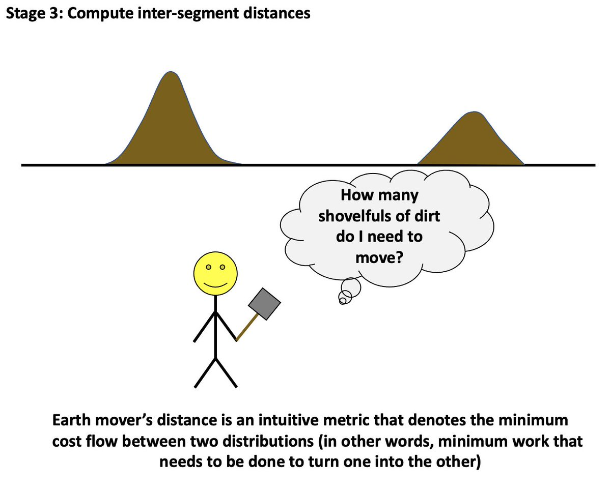
Imagine piles of dirt here to be $P_{\hat{X}}$ and $P_X$ to be a pile of dirt shaped like a bell curve. The minimum transport plan just tells you the best plan to shovel dirt in between the two piles such that the final pile resembles $P_X$.

But how does shoveling dirt relates to redistributing distributions? Every joint distribution between the two distributions $P_{\hat{X}}$ and $P_X$ can be written as a table whose each row and column sum to 1.

	$x_1$	$x_2$	$\dots$	$x_k$
${\hat{x}}_1$	$0.1$	$0.6$	$\dots$	$0.05$
${\hat{x}}_2$	0.3	0.2	$\dots$	0.3
$⋮$	$⋮$	$⋮$	$⋮$	$⋮$
${\hat{x}}_k$	0.9	0.1	$\dots$	0

This joint distribution between the two marginals $P_X$ and $P_{\hat{X}}$ is a transport plan which tells how one of the marginals can be transformed into the other. To quantify the “effort” required in a transport plan, we can use the concept of work done ($W=F\times d$ ) from Physics. In our context -

$$\begin{array}{rl}||x-\hat{x}|{|}_2& :\text{distance moved}\\ \lambda (x,\hat{x})& :\text{amount of mass moved}\\ \lambda (x,\hat{x})\cdot ||x-\hat{x}|{|}_2& :\text{"work done" in moving the mass}\end{array}$$

The average work done required in a transport plan is -

$$\begin{array}{rl}& {\int }_{X,\hat{X}}\lambda (x,\hat{x})\cdot ||x-\hat{x}|{|}_{2}dxd\hat{x}\\ & =\underset{\lambda (x,\hat{x})}{\mathbb{E}}[||x-\hat{x}|{|}_2]\end{array}$$

Let $\Pi (X,\hat{X})$ be the family of all joint distributions/transport plans between the marginals $P_X$ and $P_{\hat{X}}$ We are interested in finding the transport plan which requires the least amount of work done -

$$\underset{\lambda \in \Pi (X,\hat{X})}{\min }[\underset{\lambda (x,\hat{x})}{\mathbb{E}}||x-\hat{x}|{|}_2]$$

This is the Wasserstein’s Metric.

How to minimize Wasserstein’s Metric

The Wasserstein’s Metric is a minimization problem. Every minimization problem has a dual maximization problem. One such result of min-max duality is the Kantrovic-Rubenstein’s Duality states -

$$\begin{array}{rl}W(P_x||P_{\theta })& =\underset{||T_w(x)|{|}_L<1}{\max }[\underset{P_X}{\mathbb{E}}[T_w(x)]-\underset{P_{\theta }}{\mathbb{E}}[T_w(\hat{x})]]\\ ||T_w(x)|{|}_L& <1:\text{1-Lipschitz}\end{array}$$

Any function $f$ being 1-Lipschitz means that the function cannot change faster than the distance -

$$\frac{||f(x_1)-f(x_2)||}{||x_1-x_2||}<1$$

The $T_w$ in this case is a neural network and can be made 1-Lipschitz by normalizing the weights of $T_w$ such that $||w|{|}_2=1$ after each gradient step.

${\theta }^{\ast }$ has to be such that the Wasserstein’s distance is to be minimized. The Kantrovic-Rubenstein’s Duality enables us to express the Wasserstein’s distance in terms of expectations of $P_X$ and $P_{\theta }$.

$${\theta }^{\ast },w^{\ast }=\arg \underset{\theta }{\min }\underset{||T_w(x)|{|}_L<1}{\max }[\underset{P_X}{\mathbb{E}}[T_w(x)]-\underset{P_{\theta }}{\mathbb{E}}[T_w(\hat{x})]]$$

The above objective is very similar to GANs. That’s why this method of minimizing the Wasserstein’s metric is called the WGAN. Training a WGAN is more stable than training a Naive-GAN.

Bi-Directional GAN (Bi-GAN)

Inversion of GANs

We train a GAN specifically to allow us to sample $x$ from the dataset distribution $P_X$ by picking a random sample $z$ from an arbitrary distribution $Z$ and passing it through the generator $g_{\theta }$. But how can we get back $z$ if we know $x$?

Inversion is useful for -

1. Feature Extraction - Knowing any sample $x$ and the inversion of our GAN can allow us to obtain GAN-inverted vectors and use them as features for the data.
2. Data Manipulation/Editing - Suppose a GAN is trained on images. If we wish to edit an image using the GAN itself, we need to know the corresponding latent vector (input vector $z$) for that image and edit this vector in such a way that the image corresponding to this edited input is our desired output image.

Bi-Directional GAN

In Bi-GAN, in addition to the generator and the discriminator networks there’s also the Encoder/Inverter network denoted as $E_{\varphi }:X\to Z$.

Here the discriminator won’t just take $x$ and $g_{\theta }(z)$ as the inputs to distinguish between but take a pair of values $(x,E_{\varphi }(x))$ and $(g(z),z))$ as the input and attempt to distinguish the joint pairs. If the discriminator fails to do so, we can say that $(x,E_{\varphi }(x))\sim (g(z),z)$.

The objective function is -

$$\begin{array}{rl}{L}_{BiGAN}(\theta ,w,\varphi )& =\underset{x\sim P_X}{\mathbb{E}}[\underset{\hat{z}\sim P_{\varphi }}{\mathbb{E}}[log{D}_w(x,E_{\varphi }(x))]]+\underset{z\sim Z}{\mathbb{E}}[\underset{\hat{x}\sim P_{\theta }}{\mathbb{E}}[log\{1-D_w(x,E_{\varphi }(x))\}]]\\ {\theta }^{\ast },w^{\ast },{\varphi }^{\ast }& =\arg \underset{\theta ,\varphi }{\min }\underset{w}{\max }{L}_{BiGAN}(\theta ,w,\varphi )\\ \text{where, }& z\sim Z,\hat{x}\sim P_{\theta },\hat{z}\sim P_{\varphi }\end{array}$$

Here $g_{\theta }$ and $E_{\varphi }$ are trained simultaneously using the discriminator. Once train $g_{{\theta }^{\ast }}$ acts as the generator and $E_{{\varphi }^{\ast }}$ is used for inversion. It can be shown that,

$$\begin{array}{rl}{P}_{\hat{Z}X}& =P_{Z\hat{X}}\text{ where,}\\ P_{\hat{Z}X}& ={\int }_X{P}_X(x){\int }_{\hat{Z}}{P}_{\varphi }(\hat{z}|x)d\hat{z}dx\\ P_{Z\hat{X}}& ={\int }_Z{P}_Z(x){\int }_{\hat{X}}{P}_{\varphi }(\hat{x}|z)d\hat{x}dz\end{array}$$

Domain Adversarial Networks

Suppose we have a source dataset and target dataset such that both belong to a different distribution.

$$\begin{array}{rlr}{D}_s& =\{(x_i,y_i){\}}_{i=1}^n& \sim P_s\\ D_t& =\{({\hat{x}}_j){\}}_{j=1}^m& \sim P_t\end{array}$$

Any classifier/regressor trained solely on $D_s$ would fail to predict for the target items in $D_t$. We can use Domain Adversarial Networks here to train a classifier that is domain agnostic (able to classify independent on which domain element belong to).

In Domain Adversarial Networks we have -

1. An Encoder $\varphi :X\to F$ to extract features from inputs regardless of which domain the inputs belong to (both $D_s$ and $D_t$).
2. A Discriminator $T_w:F\to [0,1]$ to distinguish between elements of $P_s$ and elements of $P_t$ (Features of both source and target data).
3. A Classifier/Regressor $h_{\psi }:F_s\to y_s\sim P_s(y|x)$ which uses the features of the source inputs to make a prediction regarding them.

Here the Discriminator makes the Encoder better at constructing features from the inputs (both source and target) in such a way that the features appear domain agnostic. But just having domain agnostic features isn’t all, they need to be useful for predicting the target class. For this we include a Classifier/Regressor as well in the network so that the features learnt are both domain agnostic and useful.

$$\begin{array}{rlr}{\varphi }^{\ast },w^{\ast }& =\arg \underset{\varphi }{\min }\underset{w}{\max }[\underset{P_{F_s}}{\mathbb{E}}[log{D}_w(F_s)]+\underset{P_{F_t}}{\mathbb{E}}[log(1-D_w(F_t))]]& \\ {\psi }^{\ast }& =\arg \underset{\psi }{\min }\mathrm{BCE}(y,h_{\psi }(F_s))(\text{BCE=Binary Cross-Entropy})& \end{array}$$

Evaluation of a GAN

Suppose we have some true and generated samples and we wish to evaluate whether the GAN is successful in generating samples from $P_X$. There are various methods for it, but we’d be look at an adversarial method of evaluation called Frechet Inception Distance. FID uses Wasserstein’s Metric along with Inception Network trained on Imagenet to do this evaluation.

Let -

$$\begin{array}{rl}{D}_{true}& =\{x_i{\}}_{i=1}^n\stackrel{\text{iid}}{\sim }{P}_X\\ D_{gen}& =\{{\hat{x}}_j{\}}_{j=1}^m\stackrel{\text{iid}}{\sim }{P}_{\theta }\end{array}$$

1. Take a pretrained Inception Network trained on the Imagenet dataset. Let this be denoted as $I_{\psi }$.
2. Pass $D_{true}$ and $D_{gen}$ through $I_{\psi }$ and extract the features for $D_{true}$ and $D_{gen}$ from some $l^{th}$ layer of $I_{\psi }$.

$$\begin{array}{rl}{\hat{D}}_{true}& =\{z_{true}^i{\}}_{i=1}^n\stackrel{\text{iid}}{\sim }{P}_X\\ {\hat{D}}_{gen}& =\{{\hat{z}}_{gen}^i{\}}_{j=1}^m\stackrel{\text{iid}}{\sim }{P}_{\theta }\end{array}$$

3. Compute the mean and covariance for ${\hat{D}}_{true}$ and ${\hat{D}}_{gen}$.

$$\begin{array}{rl}{\mu }_{true}& =\frac{1}{n}\sum _{i=i}^n{z}_{true}^i\\ {\Sigma }_{true}& =\frac{1}{n}\sum _{i=i}^n(z_{true}^i)\cdot (z_{true}^i{)}^T\\ \text{Similarly }& {\mu }_{gen}\text{ and }{\Sigma }_{gen}\text{ too}\end{array}$$

4. Assume that the features of the true and generated data come from a Gaussian distribution of corresponding mean and variance.

$$\begin{array}{rl}{Z}_{true}& \sim \mathcal{N}({\mu }_{true},{\Sigma }_{true})\\ Z_{gen}& \sim \mathcal{N}({\mu }_{gen},{\Sigma }_{gen})\end{array}$$

5. Calculate the Wasserstein’s Metric between $Z_{true}$ and $Z_{gen}$. This is the FID, our evaluation metric of the GAN.

$$\begin{array}{rl}\mathrm{FID}& =W(Z_{true},Z_{gen})\\ & =||{\mu }_{true}-{\mu }_{gen}|{|}_2^2+\mathrm{trace}({\Sigma }_{true}+{\Sigma }_{gen}-2({\Sigma }_{true}\cdot {\Sigma }_{gen}))\end{array}$$

$P_X$ and $P_{\theta }$ would never be equal because of the heavy amount of approximations made for VDM. The GAN trained is better if the FID is lower. Lower FID means lower distance between $P_X$ and $P_{\theta }$.