Divide And Conquer

Table of Contents

• Min or Max of an array
  • Algo 1 - Linear Search
    • Pseudocode and TC
  • Algo 2 - Using Divide and Conquer
    • Pseudocode and TC
    • Properties -
• Binary Search
  • Pseudocode and TC
• Merge Sort
  • Merging
  • Merge + Sort Time Complexity
  • Properties
  • 2-way Merge Sort
• Quick Sort
  • Partitioning
  • Sorting
  • Properties -
• Master’s Method
  • Case 1
  • Case 2
  • Case 3
• Matrix Multiplication
  • Non Divide-n-Conquer
  • Divide-n-Conquer
  • Strassen’s Method
• Long Integer Multiplication
• Questions

1. Divide the bigger problem into smaller sub-problems.
2. Solve the sub-problems and combine their results if required to get the solution of the original problem.
3. In general a problem is said to be small if it can be solved in one/two basic operations.

DnC problems are of two types -

1. Symmetric - The problem is divided into sub-problems of same sizes. $T(n)=a\ast T\left(\frac{n}{b}\right)+f(n)$
2. Asymmetric - The problem is divided into sub-problems of different sizes.$T(n)=a_1\ast T(\alpha n)+a_2\ast T((1-\alpha )n)+f(n)$ Example of Symmetric DnC -

DnC(A,1,n) {
	if Small(1,n) {
		return S(A,1,n)
	} else {
		m = Divide(1,n)
		s1 = DnC(A,1,m)
		s2 = DnC(A,m+1,n)
		Combine(s1,s2)
	}
}

Here $f(n)$ is the TC of the “Divide” and “Conquer” operations -

1. Divide is Mandatory.
2. Conquer is Optional.

Min or Max of an array

Algo 1 - Linear Search

Pseudocode and TC

MinMax(A,n) {
	min = max = A[1]
	for (i=2; i<=n; i++) {
		if (A[i] < min) {
			min = A[i]
		} else if (A[i] > max) {
			max = A[i]
		}
	}
}

The Time Complexity equation is -

$$\begin{array}{rl}T(n)& =T(n-1)+2a\\ T(2)& =2b\end{array}$$

Case	Comparisons
Best Case (In Descending Order)	$n-1$
Worst Case (In Ascending Order)	$2(n-1)$
Average Case	$\frac{3}{2}(n-1)$

Algo 2 - Using Divide and Conquer

1. Divide the array into two halves.
2. Recursively split each half until the subarray size becomes:
   • 1 element → min = max = that element
   • 2 elements → find min and max using one comparison
3. Conquer (base case):
   For each smallest subarray, compute its minimum and/or maximum directly.
4. Combine:
   • Compare the minimums of the left and right subarrays to get the overall minimum.
   • Compare the maximums of the left and right subarrays to get the overall maximum.
5. Repeat the combine step bottom-up until the results for the entire array are obtained.

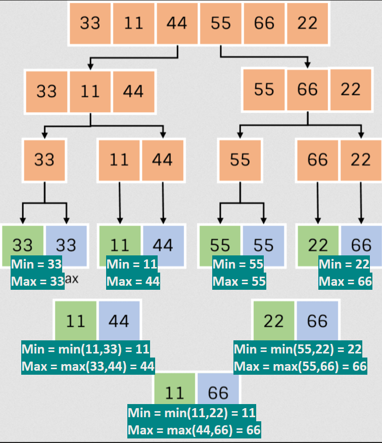
Pseudocode and TC

MinMaxDnC(i,j) {                   // Return is like (min, max)
	if (i==j) return (a[i], a[i])  // Single element sub-array 
	else if(i==j-1) {              // Double element sub-array
		if (a[i] < a[j]) {
			return (a[i], a[j])
		}
		return (a[j], a[i])
	}
 
	mid=(i+j)/2
	(min, max) = MinMaxDnC(i,mid)
	(min1, max1) = MinMaxDnC(mid+1,j)
	
	if (max1 > max) max = max1
	if (min1 < min) min = min1
	
	return (min, max)
}

The Time Complexity equation is -

$$\begin{array}{rl}T(n)& =2\ast T\left(\frac{n}{2}\right)+2a\\ T(1)& =b\end{array}$$

Case	Comparisons (Linear Search)	Comparisons (Divide n Conquer)
Best Case (In Descending Order)	$n-1$	$\frac{3}{2}(n-2)$
Worst Case (In Ascending Order)	$2(n-1)$	$\frac{3}{2}(n-2)$
Average Case	$\frac{3}{2}(n-1)$	$\frac{3}{2}(n-2)$

Properties -

1. Better worst case and average case performance than linear search.
2. Linear Search - $SC=O(1)$ Binary Search - $SC=O(lo{g}_{2}n)$ (due to the Recursion Stack)

Binary Search

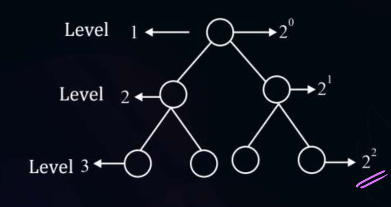The maximum number of nodes at any $i^{th}$ level of the Binary Tree is - $2^{i-1}$ Total nodes in a Binary Tree of height $h$ -

$$\begin{array}{rl}& =2^0+2^1+\cdots +2^{h-1}\\ & =\frac{1}{2}\sum _{i=0}^h{2}^i\\ & =\frac{1}{2}\ast \frac{2(2^h-1)}{2-1}\\ & =2^h-1\end{array}$$

Using this we can also find the height of a binary tree with some $n$ nodes -

$$\begin{array}{rlrl}& & n& =2^h-1\\ & \Rightarrow & n+1& =2^h\\ & \Rightarrow & h& =lo{g}_2(n+1)\\ & & & \approx O(lo{g}_{2}n)\end{array}$$

Thus -

• Minimum Possible height of a binary tree - $O(lo{g}_{2}n)$
• Minimum Possible height of a binary tree - $n$

Pseudocode and TC

BinSearch(a,i,l,x) {
	if (l==i) {
		if (x==a[i]) {
			return i
		}
		return 0
	}
	
	mid = floor((i+1)/2)
	if (x==a[mid]) return mid
	else if (x<a[mid]) return BinSearch(a,i,mid-1,x)
	else return BinSearch(a,mid+1,l,x)
}

The Time Complexity equation is -

$$\begin{array}{rl}T(n)& =T\left(\frac{n}{2}\right)+a\\ T(1)& =b\end{array}$$

Case	$TC$
Best Case (element is at mid)	$\Omega (1)$
Worst Case	$O(lo{g}_{2}n)$

1. $TC=O(lo{g}_{2}n)$
2. For Recursive BinSearch $SC=O(lo{g}_{2}n)$ (Recursion Stack) For iterative BinSearch $SC=O(1)$

Merge Sort

The idea is two merge two sorted sub-arrays to make a larger sorted array.

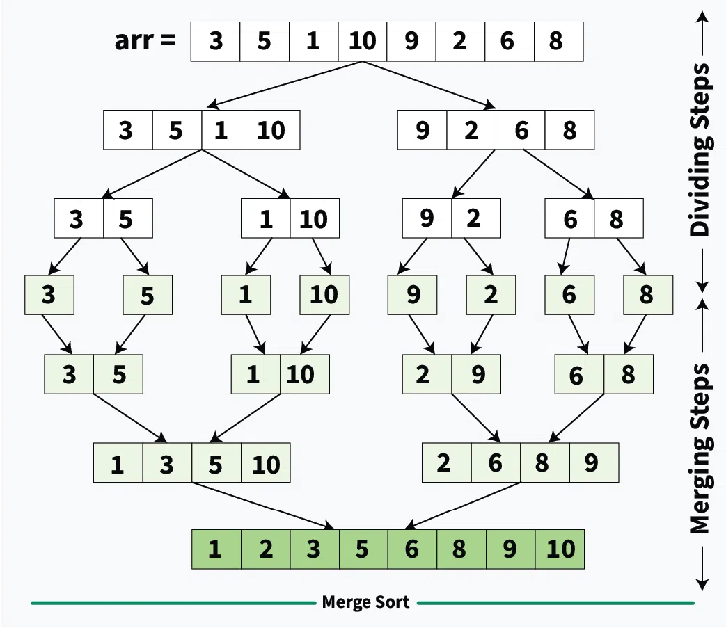
Merging

The sub-arrays are merged by using two pointers $i$ and $j$ which start from the start of each sub-array. The elements at these pointers are compared and the smaller/larger (depending upon the ordering required) one of the two is picked and that pointer is incremented.

1. Minimum number of comparisons – min(m,n) where m and n are sizes of the two sub-arrays.
2. Max number of comparisons - m+n-1 When the first m-1 elements of the L1 are smaller than the first element of L2 but the last element of L1 is greater than last element of L2.

So $TC=\Theta (n)$ for merging.

Merge + Sort Time Complexity

def merge_sort(A):
  size = len(A)
  if size <= 1:
    return A
 
  mid = size//2
  s1 = merge_sort(A[0:mid])
  s2 = merge_sort(A[mid:])
 
  i = j = 0
  m, n = len(s1), len(s2)
  temp = []
 
  while True:
    if i == m:
      temp.extend(s2[j:])
      break
    elif j == n:
      temp.extend(s1[i:])
      break
    elif s1[i] < s2[j]:
      temp.append(s1[i])
      i+=1
    elif s2[j] < s1[i]:
      temp.append(s2[j])
      j+=1
 
  return temp

The merge sort algorithm firstly divides the array into subarrays and then performs the merge operation on them. Thus the $TC$ is like -

$$\begin{array}{rlr}TC& =2\ast T\left(\frac{n}{2}\right)+\Theta (n)& \because \Theta (n)\text{ is for the merge operation}\\ & =2\ast T\left(\frac{n}{2}\right)+b\ast n& \\ & =2\ast \left(2\ast T\left(\frac{n}{4}\right)+b\ast \frac{n}{2}\right)+b\ast n& \\ & =2^2\ast T\left(\frac{n}{2^2}\right)+2\ast b\ast \frac{n}{2}+b\ast n& \\ & =2^2\ast T\left(\frac{n}{2^2}\right)+2\ast b\ast n& \\ & ⋮& \\ & =2^k\ast T\left(\frac{n}{2^k}\right)+k\ast b\ast n& \end{array}$$

For $\frac{n}{2^k}=1$, $k=lo{g}_{2}n$. Thus

$$\begin{array}{rl}TC& =O(n\ast 1+b\ast n\ast lo{g}_{2}n)\\ & =O(nlo{g}_{2}n)\end{array}$$

Because in Merge comparisons happen during the merge step, not during division, the number of comparisons is $\Theta (nlo{g}_{2}n)$ regardless of the input order. Hence, Merge Sort has no best case or worst case arrangement.

Case	$TC$
Best Case (element is at mid)	$\Omega (nlo{g}_{2}n)$
Worst Case	$O(nlo{g}_{2}n)$
Overall	$\Theta (nlo{g}_{2}n)$

Properties

1. Not In-place due to the need for an additional array temp of size $n$.
2. Is Stable.
3. The Recursion Stack would be of $O(lo{g}_{2}n)$ due to the division.
4. The Auxiliary memory however would be of $O(n)$ as a temporary array would be required for merge + sort results.
5. Thus total $SC=O(n)$.
6. Number of function calls during recursion - $2(n-1)$.

2-way Merge Sort

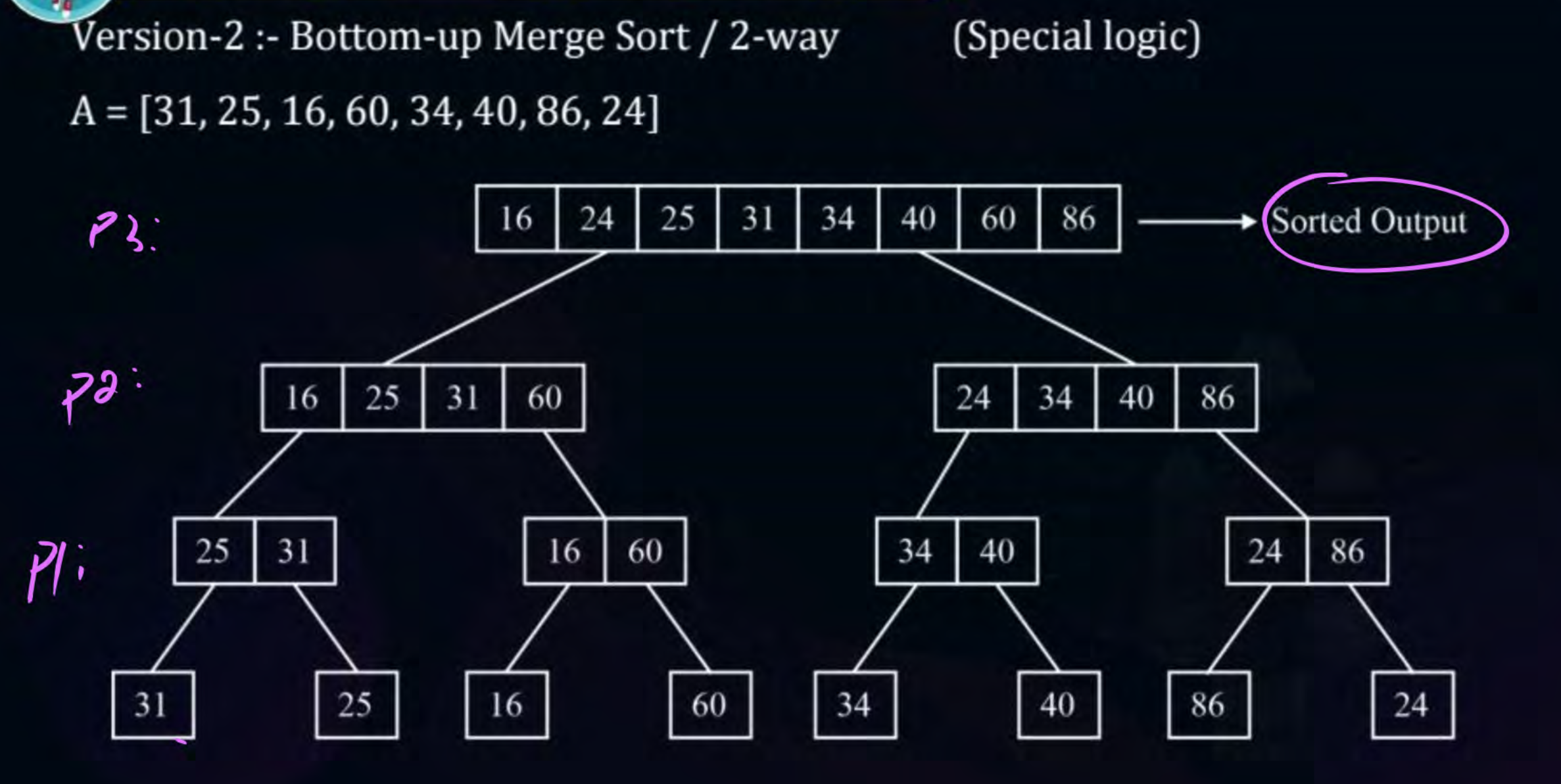
1. A variant of merge sort where we just make pairs of elements without dividing the original array from the mid. So only the “Conquer” part of Merge-Sort is done, not “Divide”.
2. Each pass processes one level of the tree.

But this might not always work as the array needs to be of length of the form of $2^k$. Example -

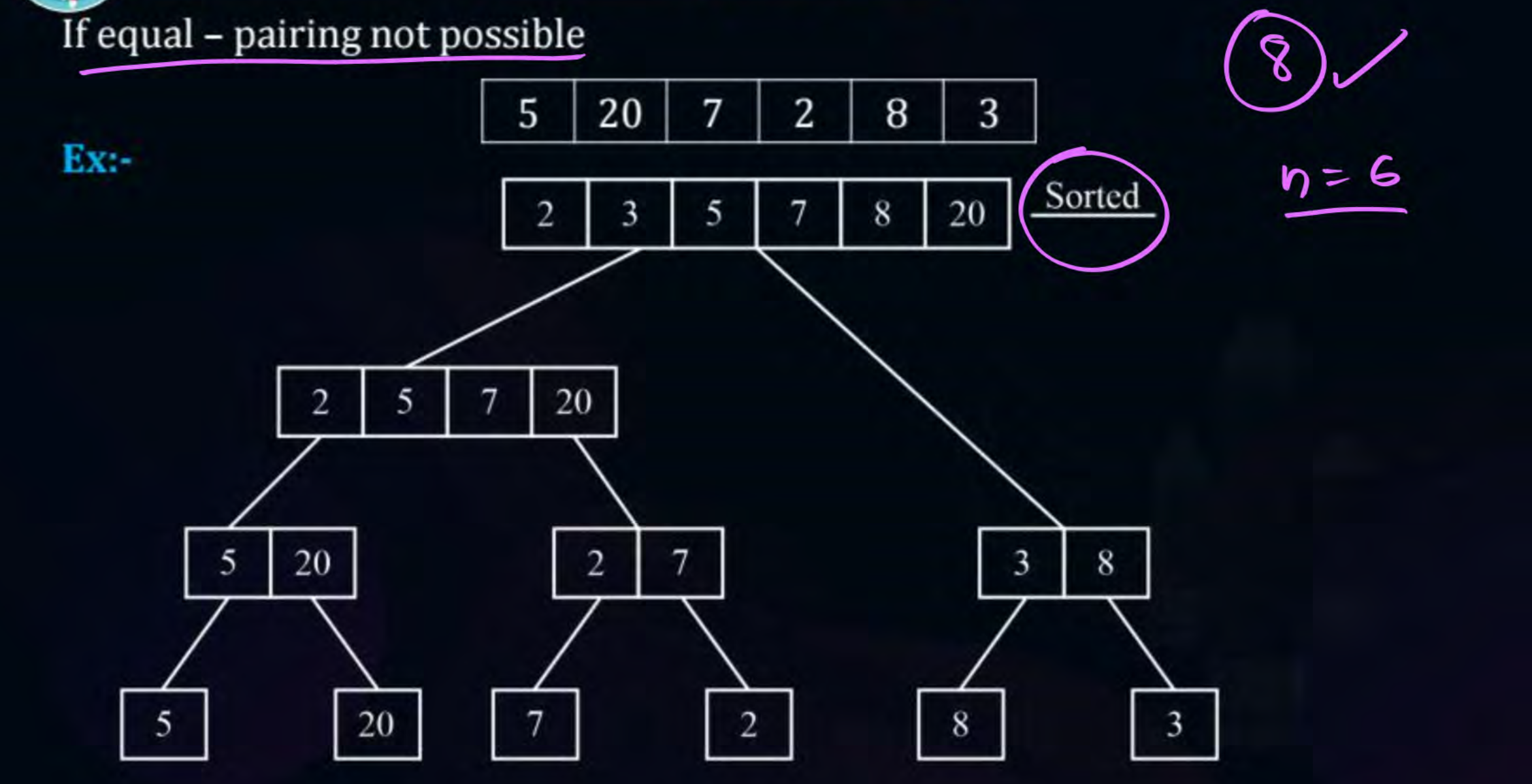
One way of solving this is by sending [3,8] up one level as it is and merging it with [2,5,7,20].

Quick Sort

Quick Sort uses a Partitioning algorithm first to partition the original array into sub-arrays. Each sub-array is then again partitioned further.

Partitioning

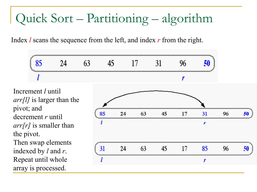
The time complexity of the partitioning algorithm would be - $O(n)$

Sorting

Best Case -

$$\begin{array}{rlr}T(n)& =T\left(\frac{n}{2}\right)+T\left(\frac{n}{2}\right)+O(n)& \because \text{Left sub-array + Right sub-array + partitioning}\\ & =O(nlo{g}_{2}n)& \text{Best Case}\end{array}$$

Worst Case -

$$\begin{array}{rlr}T(n)& =T(n-1)+O(n)& \because \text{Sub-array + partitioning}\\ & =T(n-k)+\sum _{i=1}^{k}i& \\ & =O(n^2)& \because T(1)=1\text{, thus }k=n-1\end{array}$$

Case	$TC$
Best Case (array partitions from the mid each time)	$O(nlo{g}_{2}n)$
Worst Case (when input in ascending or descending order, the partitioned sub-array will have $n-1$ elements)	$O(n^2)$

Properties -

1. Not In-place.
2. Not Stable.
3. Counter-intuitive as gives worst case for sorted inputs.
4. $SC=O(n)$ due to recursion stack.

Master’s Method

Only applicable for Symmetric DnC. Mathematically -

$$\begin{array}{rl}T(n)& =a\ast T\left(\frac{n}{b}\right)+F(n)\\ \text{Such that }& a\ge 1,b>1,F(n)=+ve\end{array}$$

1. Example - $T(n)=4T\left(\frac{n}{2}\right)+n$. Here $a=4,b=2,F(n)=n$. Thus Master’s Method applies.
2. Even when an equation might not seem to satisfy Master’s Method on the first glance, using Change of Variable might make it into an equation that would satisfy Master’s Method. See Question 3 for an example.

Case 1

If $F(n)$ is $O(n^{lo{g}_{b}a-ϵ})$ for some $ϵ>0$, then

$$T(n)=\Theta (n^{lo{g}_{b}a})$$

Case 2

If $F(n)$ is $\Theta (n^{lo{g}_{b}a}\ast (logn{)}^K)$ for some $K$, such that -

$$\begin{array}{rlrl}& (1)& K\ge 0,\text{then}& T(n)=\Theta (n^{lo{g}_{b}a}\ast (logn{)}^{K+1}))\\ & (2)& K=-1,\text{then}& T(n)=\Theta (n^{lo{g}_{b}a}\ast log(logn))\end{array}$$

Case 3

If $F(n)$ is $\Theta (n^{lo{g}_{b}a+ϵ}))$ for some $ϵ>0$, $\text{AND}$ $a\ast F\left(\frac{n}{b}\right)\le \delta \ast F(n)$, for some $\delta <1$

$$T(n)=\Theta (F(n))$$

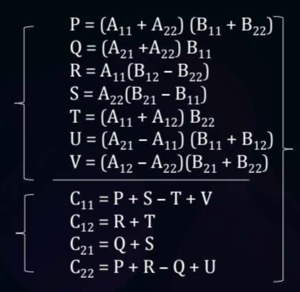
Matrix Multiplication

$$A=\left[\begin{array}{cc}{a}_{11}& a_{12}\\ a_{21}& a_{22}\end{array}\right],B=\left[\begin{array}{cc}{b}_{11}& b_{12}\\ b_{21}& b_{22}\end{array}\right],C=\left[\begin{array}{cc}{c}_{11}& c_{12}\\ c_{21}& c_{22}\end{array}\right]$$

Here $c_{11}=a_{11}\ast b_{11}+a_{12}\ast b_{21}$. Calculating one element of $C$ we need $2$ multiplications and $1$ addition. In general terms we need $m$ multiplications and $m-1$ additions to calculate one element of $C$.

Non Divide-n-Conquer

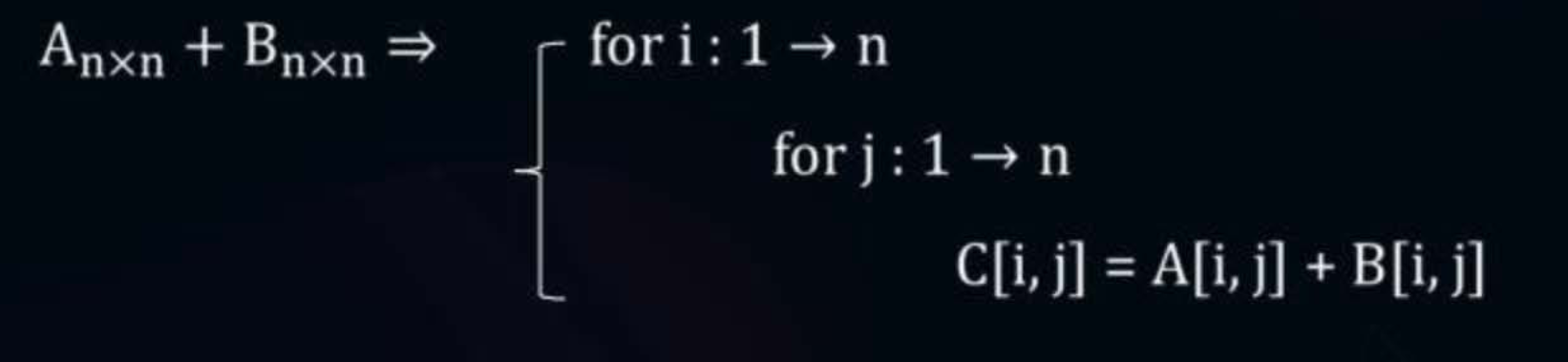
Matrix Addition -

Matrix Multiplication -

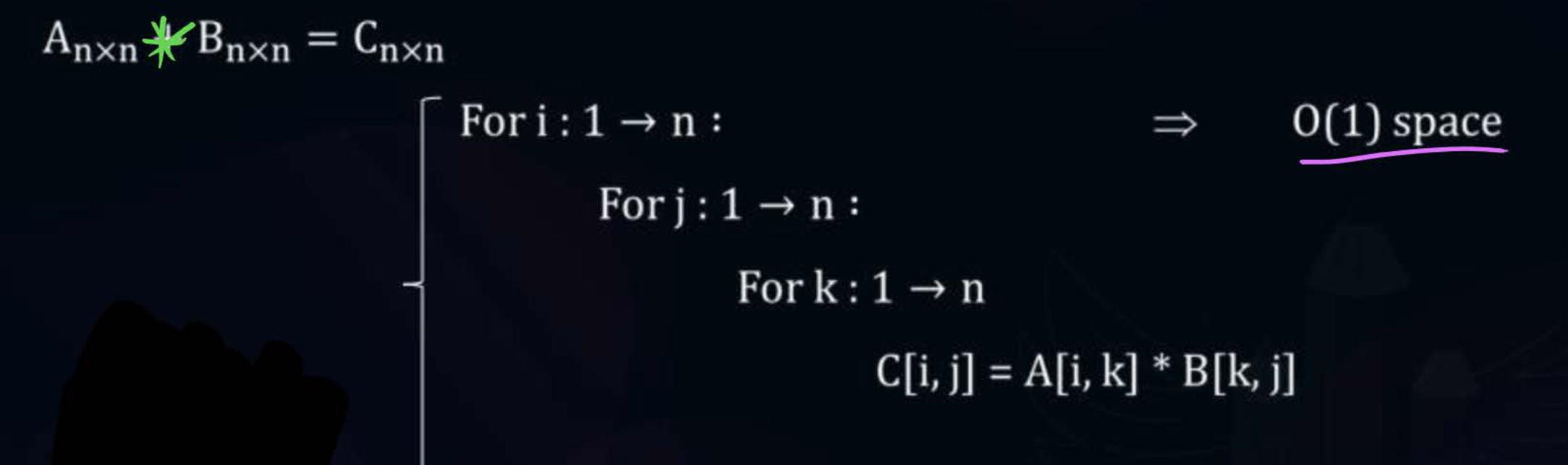
A non-DnC method of Matrix Multiplication would have TC $O(n^3)$. The TC of Matrix Addition is $O(n^2)$.

Divide-n-Conquer

We can consider a matrix of size $n\times n$ to be made up of 4 matrices of sizes $\frac{n}{2}\times \frac{n}{2}$.

$$A=\left[\begin{array}{cc}{A}_{11}& A_{12}\\ A_{21}& A_{22}\end{array}\right],B=\left[\begin{array}{cc}{B}_{11}& B_{12}\\ B_{21}& B_{22}\end{array}\right],C=\left[\begin{array}{cc}{C}_{11}& C_{12}\\ C_{21}& C_{22}\end{array}\right]$$

Here $C_{11}=A_{11}\ast B_{11}+A_{12}\ast B_{21}$, where $A_{11}\ast B_{11}$ is further a matrix multiplication between two $\frac{n}{2}\times \frac{n}{2}$ matrices.

1. If the time complexity of multiplication of two $n\times n$ matrix is $T(n)$, then time complexity of multiplication of two $\frac{n}{2}\times \frac{n}{2}$ matrix is $T(\frac{n}{2})$.
2. In calculation of $C_{11}$ we require $2$ such matrix multiplications and 1 matrix addition.
3. There are a total of $4$ such submatrices of $C$ that need to be calculated. Using the above information we can say that -

$$\begin{array}{rlr}T(n)& =4\ast 2\ast T\left(\frac{n}{2}\right)+4\ast O(n^2)& \because 4\ast O(n^2)\text{for matrix addition}\\ & =\boxed{8\ast T\left(\frac{n}{2}\right)+O(n^2)}& \\ & =\Theta (n^3)& \end{array}$$

Strassen’s Method

1. In DnC based matrix multiplication there are $8$ subproblems involved in getting $C_{11},C_{12},C_{21},C_{22}$.
2. Time complexity can be reduced if the number of subproblems is decreased from $8$.

Using this above method, by creating the matrices $P-V$, $C_{11},C_{12},C_{21},C_{22}$ can still be calculated. However now we only require $7$ subproblems instead of $8$.

$$\begin{array}{rlr}T(n)& =7\ast T\left(\frac{n}{2}\right)+b\ast O(n^2)& \\ & =\Theta (n^{lo{g}_{2}7})& \\ & \approx \Theta (n^{2.81})& \end{array}$$

Long Integer Multiplication

We use 2-way split or 3-way split and then solve. There exist 3 methods of implementing these splits -

1. Simple DnC - $T(n)=9\ast T(\frac{n}{3})+n=\Theta (n^2)$
2. AK optimization DnC - $T(n)=8\ast T(\frac{n}{3})+n=\Theta (n^{lo{g}_{3}8})\approx \Theta (n^{1.89})$
3. T&C optimization DnC - $T(n)=5\ast T(\frac{n}{3})+n=\Theta (n^{lo{g}_{3}5})\approx \Theta (n^{1.46})$

Master’s Method can be used to find the above TCs.

Coefficient of $T(\frac{n}{k})$ for some k-way split -

	Simple DnC	AK Optimization	T&C Optimization
2-way split	4	3	3
3-way split	9	8	5
4-way split	16	15	7
k-way split (generalized)	$k^2$	$k^2-1$	$2k-1$
Reccurrence Equation -

$$T(n)=c\ast T\left(\frac{n}{k}\right)+b\ast n,n>1$$

Here $c$ is the coefficient of the k-way split based upon the DnC strategy used.

---

Questions

Q1)

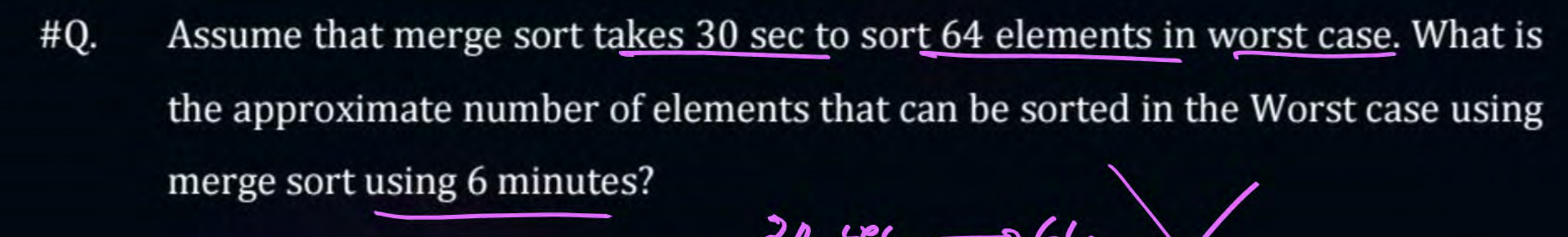
Sol${}^n$ - Here we know that the worst case time complexity for merge sort is - $O(nlo{g}_{2}n)$

$$\begin{array}{rlrl}& & 30\text{ seconds}& =c\ast nlo{g}_{2}n\\ & \Rightarrow & 30& =c\ast 64lo{g}_{2}64\\ & \Rightarrow & 30& =c\ast 64\ast 6\\ & \Rightarrow & c& =\frac{5}{64}\end{array}$$ $$\begin{array}{rlrlr}& & 6\text{ minutes}& =c\ast nlo{g}_{2}n& \\ & \Rightarrow & 360\text{ seconds}& =\frac{5}{64}\ast nlo{g}_{2}n& \\ & \Rightarrow & nlo{g}_{2}n& =4608& \\ & \Rightarrow & n& =\boxed{512}& \because \text{Hit-n-try different powers of 2}\end{array}$$

Thus for $512$ elements, merge sort would take 6 minutes in the worst case.

---

Q2)

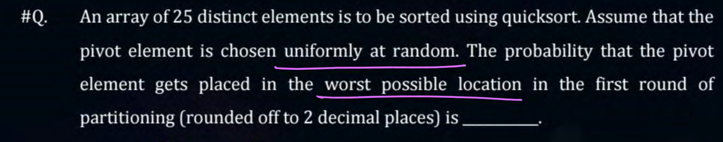
Sol${}^n$ - The worst possible positions would be either index 0 or index 24. Thus $\frac{2}{25}=\boxed{0.08}$.

---

Q3) Solve the following using Master's Method -

$$T(n)=T(\sqrt{n})+5$$

Sol${}^n$ - In its current form, the equation will not satisfy any case of the Master’s Method. We can use Change of Variable to try and convert this into an equation which will satisfy Master’s Method.

Let $n=2^k$, so $T(2^k)=T(2^{\frac{k}{2}})+5$. Let’s say for some function $S$, $S(k)=T(2^k)$. Then we can write the above equation in terms of $S$ like -

$$S(k)=S\left(\frac{k}{2}\right)+5$$

Now Master’s Method is applicable on this equation. Here $a=1,b=2,F(n)=5$. Case 2 of Master’s Method would satisfy this and thus we’d get $S(k)=\Theta (logk)$.

As $k=logn$, $T(n)=S(k)=\boxed{\Theta (log(logn))}$.

---

Q4) In a variant of Quick Sort, suppose the n/4th smallest element is picked as the pivot for partitioning. What would be the time complexity reccurrence?

Sol${}^n$ - We know that after partitioning, the pivot is placed at its correct position. Thus the ${\frac{n}{4}}^{th}$ element would be placed at the ${\frac{n}{4}}^{th}$ index of the array. The two sub-arrays that would be solved would be of size $\frac{n}{4}$ and $\frac{3n}{4}$. Thus,

$$T(n)=T\left(\frac{n}{4}\right)+T\left(\frac{3n}{4}\right)+O(n)$$

---