Dynamic Programming

Dynamic Programming is an algorithm design method used for solving problems whose solutions are viewed as a result of making a set/sequence of decisions.

• One way of making these decisions is to make them one at a time in a step-wise (sequential) manner and never make any erroneous decision.
• When applying Greedy Methods, for many problems it is not possible to make step-wise decisions based on local information available at every step in such a manner that the sequence of decisions in optimal.

Example - Using coins $C=\{1,3,4\}$ what is the minimum number of coins you can pick such that the sum is $6$ given that any coin can be picked any number of times?

• Greedy Method - $4+1+1$, thus $3$ coins
• Optimal Solution - $3+3$, thus $2$ coins

Difference between DnC and DP

1. DnC - Break up the problem into smaller and independent problems.
2. DP - Break up the problem into a series of smaller but overlapping problems.

Single Source Shortest Path (SSSP)

Djikstra’s Single Source Shortest Path

Always gives the optimal solution to the SSSP problem, provided that all edges in the graph have positive weight edges. May or may not give the optimal solution for graphs with negative weight edges.

Approaches -

1. Based on Matrix (Gives only SSSP cost not path)
2. Based on Spanning Tree (Gives both cost and path)

Matrix Based approach

In this approach we use a matrix to keep track of the total cost of reaching a certain node starting from some source node $s$.

Setup -

• The distance/cost to each node in the graph from $s$ is tracked using an array called $d$.
• The cost between any two neighbouring nodes can be found using the cost function $c$ by doing $c(n_1,n_2)$.
• We go through multiple steps by “relaxing” the node with the cheapest cost in $d$ to explore more of the graph.
• When all nodes have been relaxed and explored, we terminate the algorithm.
• Any node in the graph that isn’t reachable in the current step would have a cost of $\infty$.
• The matrix being constructed will have the value of $d$ for any $i^{th}$ step in its $i^{th}$ row.

The matrix would look like -

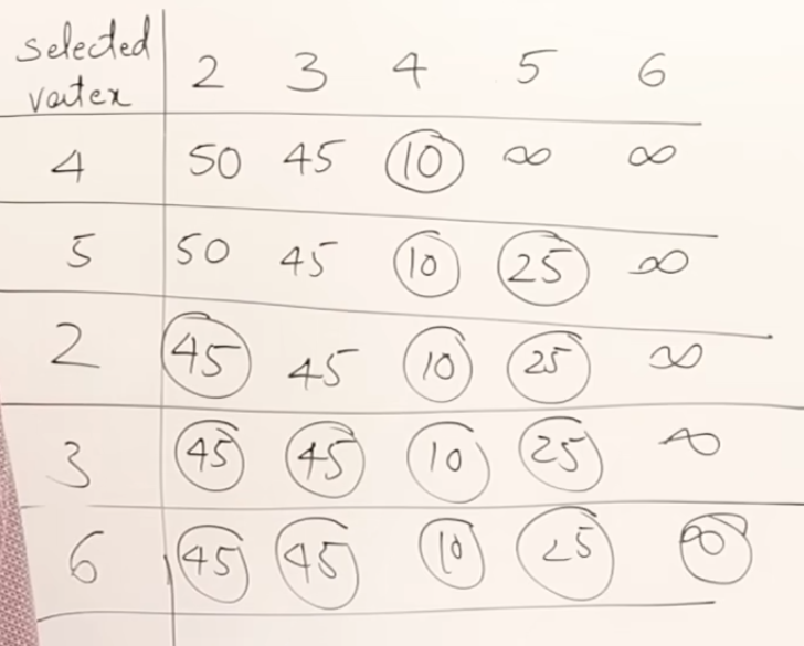
Steps -

1. Explore the source node $s$ and identify all the immediate neighbours of $s$ and their costs. As rest all nodes in the graph are unreachable at this point, they all would have a cost of $\infty$.
2. Relaxation - Identify the unexplored/unrelaxed node $v$ with the cheapest cost in the previous step. By travelling through $v$ from $s$, all neighbours of $v$ are now reachable from $s$. The cost of reaching any neighbour $w$ of $v$ will be $d[v]+c(v,w)$. Only relax if the new cost is strictly less than the old cost.

$$\begin{array}{rl}& \text{if }(d[v]+c(v,w)<d[w])\\ & \to d[w]=d[v]+c(v,w)\end{array}$$

3. Repeat Step 2. for each node in the graph. Terminate when all nodes have been relaxed.

Spanning Tree Approach

The tree obtained using this method would not be the Minimum Cost Spanning Tree.

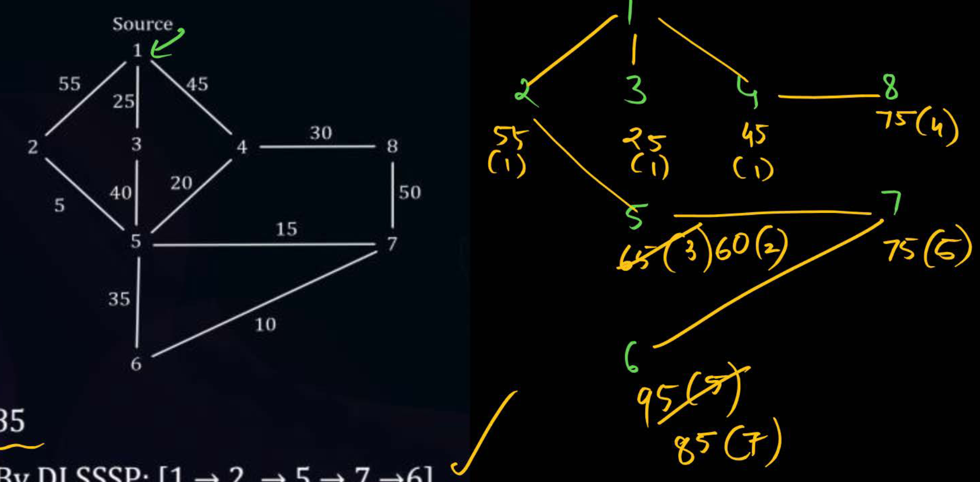
Steps -

1. Start with $s$ as the initial node $v$.
2. Explore $v$ to find the immediate neighbours. Pick the cheapest unexplored node in the graph as the new $v$ and draw a path between the node and its parent.
3. Repeat step 2 until all nodes are explored.

Time Complexity:

• $O(n^2)$ (without heap)
• $O(n+e)$ (with heap)
• If $e\approx n^2$, then $O(n^2\log n)$

Bellman-Ford algorithm

If the graph has 0 or more negative weight edges but no negative cycles, then the Bellman-Ford algorithm guarantees an optimal solution to the SSSP problem. If a graph has a negative cycle, then no algorithm would work.

Setup -

• The graph has $n$ nodes and $e$ edges.

Steps -

1. Take each edge one by one and relax it. This is one cycle.
2. Continue doing such cycles until the costs don’t change anymore. Only do a maximum of $n-1$ cycles.
3. If the costs still update after doing $n-1$ cycles (i.e the $n^{th}$ cycle), then the graph has a negative cycle and the SSSP for it cannot be solved.

Time Complexity:

• $O(n\ast e)$
• $O(n^3)$ (if the graph is a complete graph as $e=O(n^2)$)

All Pairs Shortest Path (ASSP)

Floyd-Warshall’s Algorithm

Djikstra’s SSSP algorithm can be used to calculate ASSP as well with a TC of $O(n^3)$. But it won’t be able to find the optimal ASSP solution for graphs with negative edges. That’s why we use Floyd-Warshall’s Algorithm as it can handle negative edges.

Setup -

1. Let there be $n$ nodes in the graph where $V=\{v_i{\}}_{i=1}^n$ is the set of all nodes/vertices.
2. Have an adjacency matrix $A^0$ of size $n\times n$ which shows the cost of accessing any node’s immediate neighbours. Any node that isn’t an immediate neighbour of a node will a cost of $\infty$.

Steps -

1. Start with $k=1$.
2. If $k\le n$, using $A^{k-1}$ construct an new adjacency matrix $A^k$ where any $(i,j{)}^{th}$ holds the cost of reaching $j$ from $i$ via $v_k$. This can be done by doing -

$$A^k[i][j]=\min (A^{k-1}[i][j]),A^{k-1}[i][v_k]+A^{k-1}[v_k][j])\forall (i,j)\in V\times V$$

3. Increment $k=k+1$ and repeat Step 2 until $k>n$.
4. The final adjacency matrix $A^{v_k}$ will hold the costs of the shortest paths for all pair of vertices in the graph.

Time & Space Complexity -

1. Time Complexity - $O(n^3)$
2. Space Complexity - $O(n^2)$

0/1 Knapsack (Binary Knapsack)

Unlike the Fractional Knapsack Problem, in Binary Knapsack an item can either be entirely included or entirely excluded. The objective is to maximize the profit by picking items in such a way that their total weight doesn’t exceed the Knapsack capacity.

For such a problem the recurrence algorithm is -

$$\begin{array}{rlr}01Knap(n,M)& =0,& \text{if}n=0\text{ or }M=0\\ 01Knap(n,M)& =01Knap(n-1,M),& w_n>M\\ 01Knap(n,M)& =\max \{01Knap(n-1,M),01Knap(n-1,M-w_n)+p_n\}& \end{array}$$

This means -

1. If weight of object ($w_n$) is more than the Knapsack Capacity, exclude the object.
2. If the weight of the object is less than the Knapsack Capacity, consider two cases where you can either include the object in the Knapsack or you can exclude the object from the Knapsack. Compare the Knapsack profits in both cases and pick the largest one.

Tabulation Method

Better than following textual notes regarding this, it’s better to follow the procedure demonstrated by Mr. Abdul Bari. This method can be easily implemented as a Bottom-Up Iterative solution for solving 0/1 Knapsack.

Complexity -

1. Time Complexity - $O(n\ast M)$
2. Space Complexity - $O(n\ast M)$

Sum of Subsets (SOS)

For such a problem the recurrence algorithm is -

$$\begin{array}{rlr}\mathrm{SOS}(n,M)& =\mathrm{SOS}(n-1,M)\text{ or }\mathrm{SOS}(n-1,M-A_n)& ,A_n\le M\\ \mathrm{SOS}(n,M)& =\mathrm{SOS}(n-1,M)& ,A_n>M\\ \text{Base Condition}& -& \\ & \mathrm{SOS}(n,M)=\text{False}& ,n=0\&M>0\\ & \mathrm{SOS}(n,M)=\text{True}& ,M=0\&n\ge 0\end{array}$$

Longest Common Subsequence (LCS)

A subsequence of a string is made by deleting some or none characters from the string, while keeping the order in which the characters occurs.

A substring of a string is a subsequence of a string made using contiguous characters.

Example - In abdace and babce, bace and abce are two substrings of length 4.

There are $2^n$ subsequences possible for a string of $n$ characters. So a brute force algorithm will take have the time complexity of $O(2^n)$.

Pseudocode -

LCS(A,B) {
	// of size mxn
	mem_table = [[0 for (i=0;i<=len(A);i++)] for (j=0;j<=len(B);j++)]
 
	for (i=0;i<=len(A);i++) {
		for (j=0;j<=len(B);j++) {
			if (A[i] == B[j]) {
				mem_table[i][j] = 1 + mem_table[i-1][j-1]
			} else {
				mem_table[i][j] = max(mem_table[i-1][j], mem_table[i][j-1])
			}
		}
	}
}

How the tabulation method looks like on paper. To follow this, watch Mr Abdul Bari solve it -

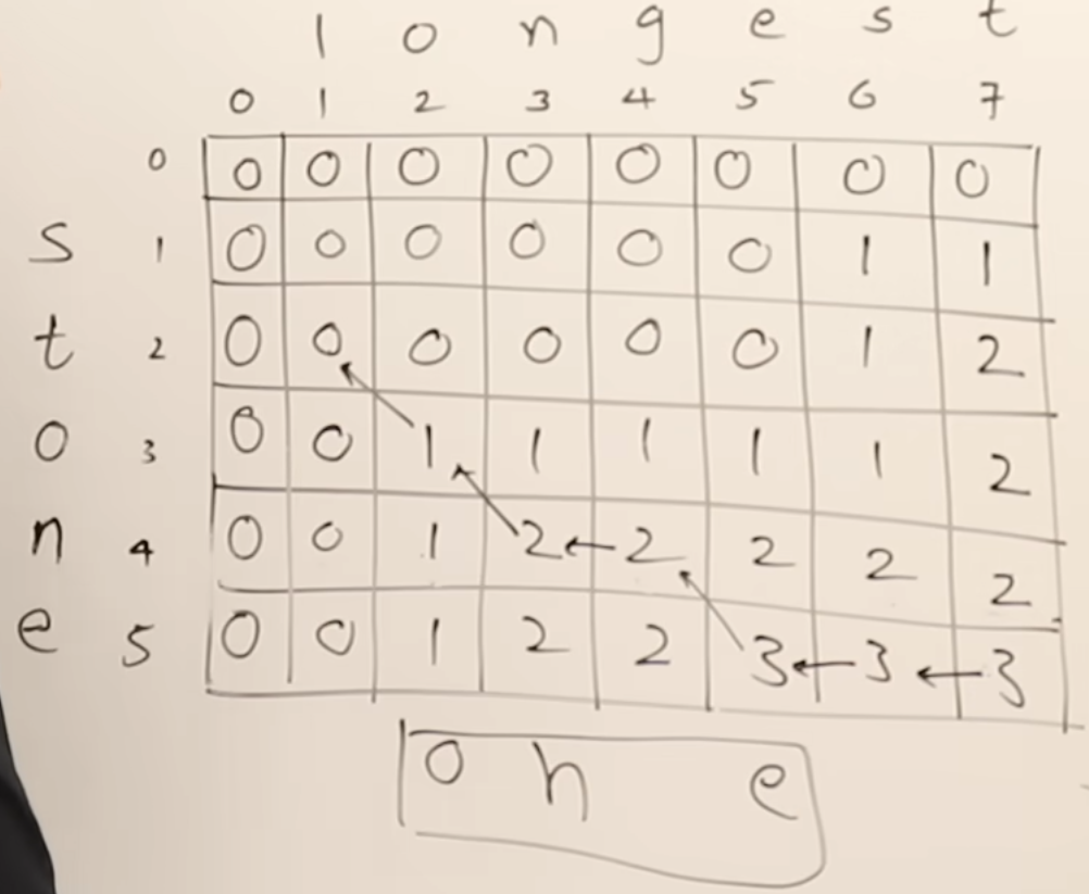
Here we are attempting to find the LCS for “longest” and “stone”.

Complexity -

1. Time Complexity - $O(m\ast n)$
2. Space Complexity - $O(m\ast n)$

Matrix Chain Multiplication (MCM)

Let $A$ and $B$ be two matrices of sizes $m\times n$ and $n\times p$. The number of scalar multiplication required in the matrix multiplication $AB$ is $m\times n\times p$.

So say we have multiple matrices like $A,B,C,D$. Their matrix product $ABCD$ can be achieved by multiplying the matrices in any order, either by doing $A(BCD)$ or $(AB)(CD)$ or $(ABC)D$. MCM attempts to find the optimal order in which the matrices should be multiplied to minimize the amount of scalar multiplication required.

The number of ways to parenthesize the multiplication of $n$ matrices corresponds to the number of full binary trees with $n$ leaves (each leaf representing a matrix).

This number is given by the Catalan number -

$$C_{n-1}=\frac{1}{n}\left(\genfrac{}{}{0ex}{}{2n-2}{n-1}\right)$$

Each such binary tree represents a distinct order of matrix multiplication.